Linear, Convolution

매일 공부(ML)·2021년 10월 27일

CS

목록 보기

17/33

학습 목표

레이어 개념
레이어 동작 방식
레이어 설계
Tensorflow 정의

데이터 형태

(m,n) 행렬 -> dataframe
(C,W,H) -> Channel , Width, Height
Channel : 이미지 데이터

Layer

정의: 하나의 물체가 여러 개의 논리적인 객체로 구성.

Linear Layer

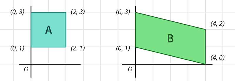
정의: 선형변환과 동일한 기능을 한다.
특징

1.선형변환을 통해서 특정 차원으로 데이터 변환
- 데이터가 풍부해지거나 집약시키는 효과가 있음.
  
  2.(a,b) and (a* b) 모두 같은 행렬이다.
  
  3.각각의 행렬들은 Weight
  
  4.Weight의 모든 요소는 Parameter
  
  5.Parameter의존 시 과적합이 일어난다.
  
  6.적합한 Weight찾기 <-- 훈련!!
  
  7.지역성 자체가 엄청 중요한 정보.
  
  -> 만약 삭제되었을 경우 입출력 사이의 관계 가중치를 찾아야한다.
꼴: (입력의 차원, 출력의 차원)
bias(편향)
- 정의: 선형변환된 값에 편향 파라미터를 더해주는 것이다.
목적: 데이터별로 맞는 Weight 선언하자!

코드로 구현 1탄

## 데이터 집약시키는 코드

import tensorflow as tf

batch_size = 64
boxes = tf.zeros((batch_size, 4, 2))     # Tensorflow는 Batch를 기반으로 동작하기에,
                                         # 우리는 사각형 2개 세트를 batch_size개만큼
                                         # 만든 후 처리를 하게 됩니다.
print("1단계 연산 준비:", boxes.shape)

first_linear = tf.keras.layers.Dense(units=1, use_bias=False) 
# units은 출력 차원 수를 의미합니다.


first_out = first_linear(boxes)
first_out = tf.squeeze(first_out, axis=-1) # (4, 1)을 (4,)로 변환해줍니다.
                                           # (불필요한 차원 축소)

print("1단계 연산 결과:", first_out.shape)
print("1단계 Linear Layer의 Weight 형태:", first_linear.weights[0].shape)

print("\n2단계 연산 준비:", first_out.shape)

second_linear = tf.keras.layers.Dense(units=1, use_bias=False)
second_out = second_linear(first_out)
second_out = tf.squeeze(second_out, axis=-1)

print("2단계 연산 결과:", second_out.shape)
print("2단계 Linear Layer의 Weight 형태:", second_linear.weights[0].shape)

코드 구현 2탄

## 데이터 풍부

import tensorflow as tf

batch_size = 64
boxes = tf.zeros((batch_size, 4, 2))

print("1단계 연산 준비:", boxes.shape)

first_linear = tf.keras.layers.Dense(units=3, use_bias=False)
first_out = first_linear(boxes)

print("1단계 연산 결과:", first_out.shape)
print("1단계 Linear Layer의 Weight 형태:", first_linear.weights[0].shape)

print("\n2단계 연산 준비:", first_out.shape)

second_linear = tf.keras.layers.Dense(units=1, use_bias=False)
second_out = second_linear(first_out)
second_out = tf.squeeze(second_out, axis=-1)

print("2단계 연산 결과:", second_out.shape)
print("2단계 Linear Layer의 Weight 형태:", second_linear.weights[0].shape)

print("\n3단계 연산 준비:", second_out.shape)

third_linear = tf.keras.layers.Dense(units=1, use_bias=False)
third_out = third_linear(second_out)
third_out = tf.squeeze(third_out, axis=-1)

print("3단계 연산 결과:", third_out.shape)
print("3단계 Linear Layer의 Weight 형태:", third_linear.weights[0].shape)

total_params = \
first_linear.count_params() + \
second_linear.count_params() + \
third_linear.count_params()

print("총 Parameters:", total_params)

Convolution Layer

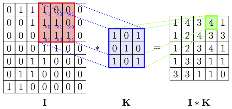
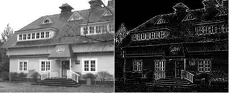
Convolution이란?

: 하나의 함수와 또 다른 함수를 곱한 후 그 구간에 대하여 적분하여 새로운 함수를 구하는 것. --> 필터와 이미지가 겹치는 부분에 Conv연산을 하면 새롭게 변형된 이미지를 얻을 수 있게 됩니다.

효과
1. image detection
2. Blur처리
- Simple box
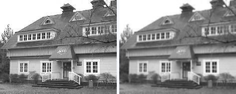
- Gaussian
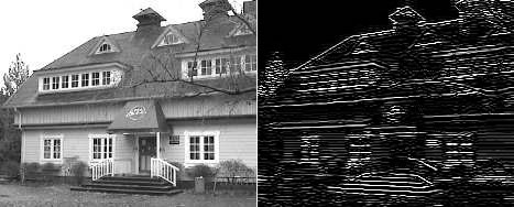
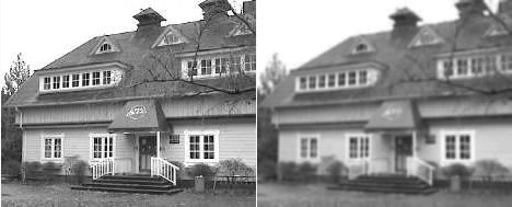
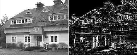
1. Edge detection
2. The Sobel Edge Operator
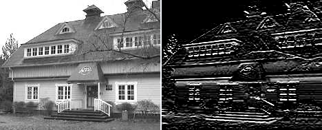
1. The laplacian operator
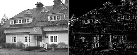
1. The Laplacian of Gaussian

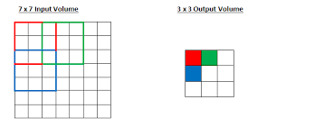
Conv 연산

: 입력의 형태를 변형시킨다.
stride: 보폭
padding쓰는 이유
1. stride가 크거나 혹은 필터가 커서 제대로Convoluation연산이 되지 않게 되는 것을 방지함.
2. 보통은 filter을 이용하면 input이미지가 작아지게 될 수밖에 없으나 zero-padding를 이용하면 이미지의 크기가 유지가 됩니다.
3. Conv이후 아웃풋 이미지 크기 유지
4. Edge쪽 픽셀정보 더 활용하기 위해서이다.
구성:[필터의 개수 필터의 가로 필터의 세로]로 이루어진 Weight.
특징
1. 입력 정보를 집약 시킴(by 여러 개의 레이어 중첩)
2. 최종 Linear가 작아져서 최적화가 가능함
3. 지역성 정보가 온전히 보전히 되기에 인접한 픽셀들 사이의 패턴만 추출하면 불필요한 연산 제거 및 정확한 계산이 가능하다.
문제점
1. 필터가 object detectino을 담기에 작을 수 있다
2. stride사이즈로 인해서 파라미터는 줄어드나 object 필터 경계선에 걸려 인식을 못할 가능성도 있다.
3. 극단적으로 필터사이즈와 이미지를 같게하면 Linear Layer가 된다. 그리고 그로 인해 연산량이 증가하여Accuracy 감소.
코드로 구현


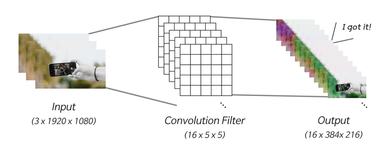
import tensorflow as tf

batch_size = 64
pic = tf.zeros((batch_size, 1920, 1080, 3))

print("입력 이미지 데이터:", pic.shape)
conv_layer = tf.keras.layers.Conv2D(filters=16,
                                    kernel_size=(5, 5),
                                    strides=5,
                                    use_bias=False)
conv_out = conv_layer(pic)

print("\nConvolution 결과:", conv_out.shape)
print("Convolution Layer의 Parameter 수:", conv_layer.count_params())

flatten_out = tf.keras.layers.Flatten()(conv_out)
print("\n1차원으로 펼친 데이터:", flatten_out.shape)

linear_layer = tf.keras.layers.Dense(units=1, use_bias=False)
linear_out = linear_layer(flatten_out)

print("\nLinear 결과:", linear_out.shape)
print("Linear Layer의 Parameter 수:", linear_layer.count_params())

Pooling Layer

Receptive Field

Process: NN이 충분한 정보를 얻기 위해 커버하는 입력데이터의 수용영역으로 이 부분이 충분히 커야하고 입력 데이터 안에 object의 특성이 포함 되어야함

MAX POOLING

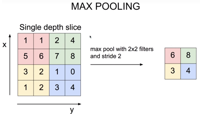
정의;효과적으로 Receptive Field를 키우고 그로 인해 정보 집약 효과가 극대화가 되고 필터 사이즈는 0입니다.
특징: 가장 큰 대표영역 뽑고 나머지는 무시합니다.

왜 MAX POOLING는 Accuracy 저하X

translational invariance효과

: 시프트 효과가 일어나도 동일한 특징을 안정적으로 잡아내어서 오버피팅 방지 및 안정적인 특징 추출 효과

비선형 함수가 갖고 있는 추출 효과를 가짐

: 하위 레이어의 연산 결과는 무시하나 상위 레이어 추출하여 올려서 성능 증진.

Receptive Field 극대화.

: 레이어를 많이 쌓으면 오버피팅, 연상량 증가, 기울기 손실등의 문제가 발생하지만 그것을 해결함.

Deconvolution Layer

Auto Encoder

정의: Convolution결과를 역재생하여 원본 복원
만드는 순서

import 패키지 and load MNIST Dataset

## 이미지 복원을 할 것이기 때문에 y_train, y_test를 사용하지 않고
## x_train의 라벨이 x_train자신이 된다.

import numpy as np
from tensorflow.python.keras.layers import Input, Dense, Conv2D, MaxPooling2D, UpSampling2D
from tensorflow.python.keras.models import Model
from tensorflow.python.keras.datasets import mnist
import json
import matplotlib.pyplot as plt #for plotting

# MNIST 데이터 로딩
(x_train, _), (x_test, _) = mnist.load_data()    # y_train, y_test는 사용하지 않습니다.

x_train = np.expand_dims(x_train, axis=3)
x_test = np.expand_dims(x_test, axis=3)

x_train = x_train.astype('float32') / 255.
x_test = x_test.astype('float32') / 255.

Auto Encoder Model 구성

# 모델 구성

# AutoEncoder 모델 구성 - Input 부분
input_shape = x_train.shape[1:]
input_img = Input(shape=input_shape)

# AutoEncoder 모델 구성 - Encoder 부분
encode_conv_layer_1 = Conv2D(16, (3, 3), activation='relu', padding='same')
encode_pool_layer_1 = MaxPooling2D((2, 2), padding='same')
encode_conv_layer_2 = Conv2D(8, (3, 3), activation='relu', padding='same')
encode_pool_layer_2 = MaxPooling2D((2, 2), padding='same')
encode_conv_layer_3 = Conv2D(4, (3, 3), activation='relu', padding='same')
encode_pool_layer_3 = MaxPooling2D((2, 2), padding='same')

encoded = encode_conv_layer_1(input_img)
encoded = encode_pool_layer_1(encoded)
encoded = encode_conv_layer_2(encoded)
encoded = encode_pool_layer_2(encoded)
encoded = encode_conv_layer_3(encoded)
encoded = encode_pool_layer_3(encoded)

# AutoEncoder 모델 구성 - Decoder 부분
# Conv2D: shape를 변화시키지 않는다.
## MaxPooling2D만 output Shape변화
decode_conv_layer_1 = Conv2D(4, (3, 3), activation='relu', padding='same')
decode_upsample_layer_1 = UpSampling2D((2, 2))
decode_conv_layer_2 = Conv2D(8, (3, 3), activation='relu', padding='same')
decode_upsample_layer_2 = UpSampling2D((2, 2))
decode_conv_layer_3 = Conv2D(16, (3, 3), activation='relu')
decode_upsample_layer_3 = UpSampling2D((2, 2))
decode_conv_layer_4 = Conv2D(1, (3, 3), activation='sigmoid', padding='same')

# upsampling2d를 거쳐서 최종 출력 28 * 28 사이즈가 나온다
#upsampling2d를 거친다
decoded = decode_conv_layer_1(encoded)   # Decoder는 Encoder의 출력을 입력으로 받습니다.
decoded = decode_upsample_layer_1(decoded)
decoded = decode_conv_layer_2(decoded)
decoded = decode_upsample_layer_2(decoded)
decoded = decode_conv_layer_3(decoded)
decoded = decode_upsample_layer_3(decoded)
decoded = decode_conv_layer_4(decoded)

# AutoEncoder 모델 정의
autoencoder = Model(input_img, decoded)
autoencoder.summary()

모델 훈련

##  이미지 생성

x_test_10 = x_test[:10]       # 테스트 데이터셋에서 10개만 골라서
x_test_hat = autoencoder.predict(x_test_10)    # AutoEncoder 모델의 이미지 복원생성
x_test_imgs = x_test_10.reshape(-1, 28, 28)
x_test_hat_imgs = x_test_hat.reshape(-1, 28, 28)

plt.figure(figsize=(12,5))  # 이미지 사이즈 지정
for i in range(10):  
    # 원본이미지 출력
    plt.subplot(2, 10, i+1)
    plt.imshow(x_test_imgs[i])
    # 생성된 이미지 출력
    plt.subplot(2, 10, i+11)
    plt.imshow(x_test_hat_imgs[i])

Decoder Layers for Reconstruction

: 실제로 역연산을 통해서 이미지를 복원

Upsampling 레이어

Nearest Neighbor : 복원해야 할 값을 가까운 값으로 복제한다.

Bed of Nails : 복원해야 할 값을 0으로 처리한다.

Max Unpooling : Max Pooling 때 버린 값을 복원한다.

Transposed Convolution

코드로 구현

from tensorflow.python.keras.layers import Conv2DTranspose

# Conv2DTranspose를 활용한  AutoEncoder 모델
# AutoEncoder 모델 구성 - Input 부분
input_shape = x_train.shape[1:]
input_img = Input(shape=input_shape)

# AutoEncoder 모델 구성 - Encoder 부분
encode_conv_layer_1 = Conv2D(16, (3, 3), activation='relu')
encode_pool_layer_1 = MaxPooling2D((2, 2))
encode_conv_layer_2 = Conv2D(8, (3, 3), activation='relu')
encode_pool_layer_2 = MaxPooling2D((2, 2))
encode_conv_layer_3 = Conv2D(4, (3, 3), activation='relu')

encoded = encode_conv_layer_1(input_img)
encoded = encode_pool_layer_1(encoded)
encoded = encode_conv_layer_2(encoded)
encoded = encode_pool_layer_2(encoded)
encoded = encode_conv_layer_3(encoded)

# AutoEncoder 모델 구성 - Decoder 부분  - 
decode_conv_layer_1 = Conv2DTranspose(4, (3, 3), activation='relu', padding='same')
decode_upsample_layer_1 = UpSampling2D((2, 2))
decode_conv_layer_2 = Conv2DTranspose(8, (3, 3), activation='relu', padding='same')
decode_upsample_layer_2 = UpSampling2D((2, 2))
decode_conv_layer_3 = Conv2DTranspose(16, (3, 3), activation='relu')
decode_upsample_layer_3 = UpSampling2D((2, 2))
decode_conv_layer_4 = Conv2DTranspose(1, (3, 3), activation='sigmoid', padding='same')

decoded = decode_conv_layer_1(encoded)   # Decoder는 Encoder의 출력을 입력으로 받습니다.
decoded = decode_upsample_layer_1(decoded)
decoded = decode_conv_layer_2(decoded)
decoded = decode_upsample_layer_2(decoded)
decoded = decode_conv_layer_3(decoded)
decoded = decode_upsample_layer_3(decoded)
decoded = decode_conv_layer_4(decoded)

# AutoEncoder 모델 정의
autoencoder = Model(input_img, decoded)
autoencoder.summary()