SSD: Single Shot MultiBox Detector

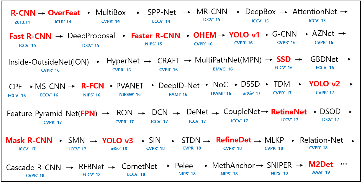
오늘 리뷰할 논문은 OverFeat, MultiBox, SPPNet, YOLO처럼 1-stage object detection을 하는 SSD 논문이다.

아래 포스트를 먼저 읽으면 도움이 될 것이다.

• SSD 논문(SSD: Single Shot MultiBox Detector) 리뷰
• 논문 리뷰 - SSD(Single Shot MultiBox Detector) 톺아보기

---

Summary

현재(당시) SOTA object detection system들은 bounding boxes를 hypothesize한 후, 각 box마다 pixel이나 feature를 재조정한 후 high quality classifier을 적용하는 접근을 취했다.

이 방식이 정확도는 높지만, embedded systems에겐 연산이 부담되고 high-end hardware조차 real-time application을 하기엔 느리다.

이 논문은 pixels이나 features를 resample하지 않고도 기존의 모델만큼이나 정확한 object detector을 선보인다. bounding box proposals과 뒤따르는 pixel/feature resampling stage를 제거함으로써 근본적인 속도 향상을 이루었다.

기존에도 이런 시도는 있었지만, 그것들과 달리 이 논문은 정확도도 높다. 논문은 bounding box locations에서 사물의 categories와 offsets을 예측하기 위해 작은 convolutional filter를 사용하고, 서로 다른 aspect ratio detection에서 서로 다른 predictors (filters)를 사용하며, multiple scales에서 detection하기 위해 network의 later stages에서 이 filter들을 multiple feature maps에 적용한다. 이 방법을 통해(특히 서로 다른 scale의 prediction을 위해 multiple layers를 사용하는 방식을 통해) 상대적으로 낮은 resolution input으로도 높은 high-accuracy와 빠른 detection speed가 모두 가능하다.

요약은 아래와 같다.

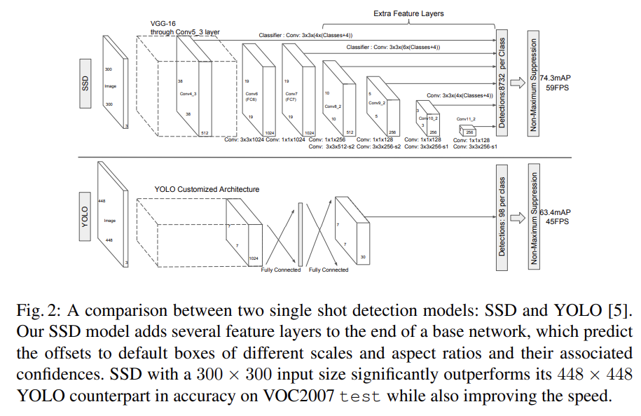
Single Shot Detector (SSD)는 bounding boxes의 fixed-size collection과 그 boxes 내에 object class가 존재하는지 score을 생성하는 feed-forward convolutional network이며 NMS 단계에서 최종 detection을 형성한다. early network(=base network)는 기존에 존재하던 architecture에서 classification layers를 잘라 사용하고, 거기에 auxiliary structure를 추가해 곧 설명할 핵심 features를 가지게 한다.

• Multi-scale feature maps for detection
  truncated base network의 끝에 convolutional feature layers를 추가한다. 이 layer들은 점진적으로 크기가 작아지고 multiple scale에서 detection을 가능하게 한다. 각 feature layers마다 convolutional model의 종류가 다르다.

• Convolutional predictors for detection
  추가된 각 feature layer는 set of convolutional filters를 사용해 fixed set of detection predictions를 생성할 수 있다. p channels을 가진 m x n feature layer에 3 × 3 × p small kernel를 적용해 category에 대한 score이나 default box 좌표에 상대적인 shape offset를 생성한다.

• Default boxes and aspect ratios
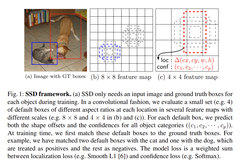
  network 꼭대기(top)에 있는 multiple feature maps에 대해 각 feature map cell마다 set of default bounding boxes를 연관시킨다. default boxes는 convolutional한 방식으로 feature map과 겹쳐지기(tile) 때문에 상응하는 cell에 대한 각 box의 상대적인 위치는 고정되어 있다. 각 cell마다 default box shapes에 상대적인 offset과 각 boxes 내의 per-class scores를 계산한다. 즉 어떤 location에 k boxes가 있고 c classes와 4 offset이 있으면 m x n feature map의 location마다 (c + 4)k filter가 적용되어 (c + 4)kmn outputs를 만들게 된다.

default box는 Faster R-CNN의 anchor box와 유사하지만, 여기서는 다른 resolution을 가진 여러 feature maps에 적용한다는 점에서 다르다. 이는 space of possible output box shapes를 효과적으로 discretize하게 한다.

training 시에 어떤 default box가 ground truth에 해당하는지 결정해야하므로 최고의 jaccard overlap를 가진 box를 선택했다. 그리고 default boxes를 jaccard overlap이 threshold(0.5)보다 높은 아무 ground truth와 match했다. 이는 network가 maximum overlap를 가진 하나만 고르는 게 아니라 multiple overlapping default boxes에 대해 높은 scores를 예측하게 한다.

training objective는 MultiBox objective [7,8]에서 유래했지만 multiple object categories를 다루기 위해 확장되었다. $x^p_{ij}$ = { 0, 1 }는 category p에서 i번째 default box와 j번째 ground truth box가 match되는지 여부를 의미한다. loss function은 localization loss(loc)와 confidence loss(conf)의 가중합이다. N은 match된 default boxes의 수고, N=0이면 loss=0으로 둔다.

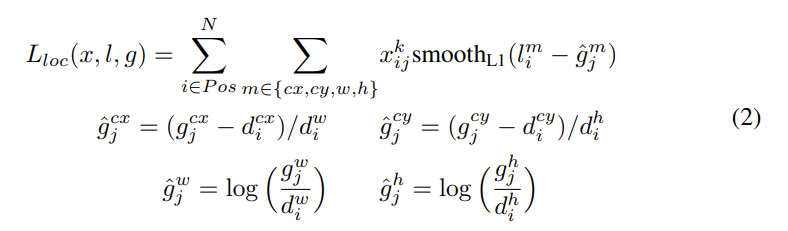
loc은 predicted box (l)와 ground truth box (g) parameters 사이의 Smooth L1 loss이다. default bounding box (d)의 중앙 offset (cx, cy)와 width (w), height (h)를 regress한다.

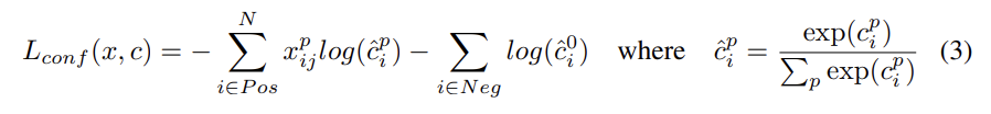
confidence loss는 multiple classes confidences (c)에 대한 softmax loss이고 weight term α는 cross validation을 통해 1로 set된다.

기존엔 여러 크기의 input을 넣고 result를 결합해서 다양한 object scale을 다뤘는데, 이 논문은 여러 layer에서의 feature map을 활용해 같은 효과를 낸다.

SSD에서 default box는 각 layer의 실제 receptive field와 꼭 일치할 필요는 없다. tiling of default boxes는 특정 feature maps가 특정 scales에 responsive하게 학습하도록 디자인되었다. m feature maps를 사용할 때 각 feature map의 default box의 scale은 다음과 같이 계산된다.

$s_{min} = 0.2, s_{max} = 0.9$인데 이는 lowest layer가 scale 0.2, highest layer가 sclale 0.9고 중간의 layer들은 같은 간격으로 있다는 것이다. default boxes에 대해 여러 aspect ration $a_r$={ 1, 2, 3, 1/2, 1/3 }을 할당하고 각 default box의 width $w^a_k = s_k \sqrt{a_r}$와 height $h^a_k = s_k / \sqrt{a_r}$을 계산할 수 있다. 특히 aspect ratio 1에 대해서는 scale이 $s_k' = \sqrt{s_k s_{k+1}}$인 default box도 추가해 feature map location마다 총 6개의 default box를 할당한다.

matching step 이후 대부분의 default box는 negative인데, 이는 positive/negative training example 간 심각한 불균형을 초래한다. 그래서 모든 negative example을 사용하는 대신 각 default box마다 높은 confidnece loss를 가진 순서로 정렬해서 negative : positive 비율이 3 : 1이 되도록 loss가 높은 순으로 뽑는다. 이런 Hard negative mining은 더 빠른 optimization과 stable training을 가능케 했다.

또 모델이 다양한 input size와 shape에 robust하도록 Data augmentation을 한다. training image은 아래의 3 옵션 중 하나로 랜덤하게 sample된다.
1. entire original input image를 사용
2. object와 minimum jaccard overlap이 0.1/0.3/0.5/0.7/0.9가 되도록 patch를 sample
3. 랜덤하게 patch를 sample

각 샘플된 patch의 크기는 원본 이미지 크기의 [0.1, 1]이고 aspect ratio는 1/2에서 2 사이다. ground truth box의 중심이 sampled patch 내에 있으면 ground truth box와의 overlap된 부분을 냅뒀다. sampling step 이후 각 sampled patch는 fixed size로 resize되고 0.5 확률로 평행하게 flip되고 photo-metric distortions이 적용된다.

실험을 위해 Base network는 ILSVRC CLS-LOC dataset으로 pre-train된 VGG16을 사용한다. DeepLab-LargeFOV [17]처럼 fc6, fc7을 convolutional layers로 교체하고, fc6과 fc7에서 parameters을 subsample하고, pool5을 2 × 2 − s2에서 3 × 3 − s1로 바꾸고, a' trous algorithm [18]을 사용해 "holes"를 채운다. 모든 dropout layers와 fc8 layer을 제거한다. 그리고 나서 SGD로 fine-tuning한다.

Strengths

1. 여러 scale input을 사용하는 대신 여러 층에서 feature을 사용한 점이 참신했다.
2. data augmentation 전략이 mAP에 상당히 크게 기여했다. (하지만 반대로 저 전략이 없으면 SSD 자체의 정확도는 비교적 낮다고 할 수도...)
3. 2-stage object detection만큼이나 정확하면서 속도는 몹시 빠르다.

Weaknesses

1. 물체 크기에 따른 정확도가 달랐다. 작은 물체가 큰 물체보다 감지 성능이 낮다. top layer에서는 information이 적어서 작은 물체를 감지하기 힘들었다.