오늘 리뷰할 논문은 Fast R-CNN의 발전형인 Faster R-CNN이다.
아래 포스트를 먼저 보면 도움이 될 것이다.
Fast R-CNN은 여전히 region proposal computation을 속도의 bottleneck으로 가진다. 논문은 detection network와 full-image convolutional features를 공유하는 Region Proposal Network (RPN)를 소개하여 거의 cost-free한 region proposals을 가능하게 한다.
RPN은 fully convolutional network이며 각 위치에서 object bound와 objectness score을 계산한다. detection에 사용될 high-quality region proposals를 뽑아내기 위해 RPN은 end-to-end로 학습된다. 그리고 RPN과 Fast R-CNN을 convolutional feature를 공유하는 식으로 합쳐 하나의 네트워크로 만든다. 일종의 “attention” mechanisms인데, RPN component가 네트워크에 어디를 볼 지 가르쳐주는 것이다.
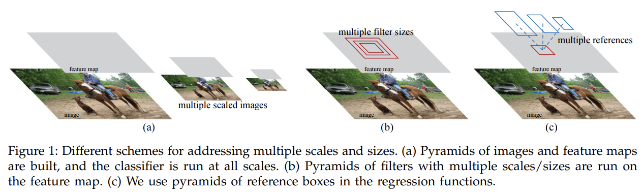
RPN은 넓은 범위의 scale과 aspect ratio에서 효과적으로 region proposal을 예측한다. 기존의 방법들은 pyramids of images나 pyramids of filters 방식을 썼는데, 여기선 새로운 'anchor' boxes라는 걸 써서 여러 scale과 aspect ratio에서 reference 역할을 한다. 이 모델은 single-scale images로도 잘 작동하므로 속도에 이점이 있다.
RPN과 Fast R-CNN을 합치기 위해서 region proposal의 fine-tuning과 object detection의 fine-tuning을 번갈아 하는 training scheme을 사용한다.
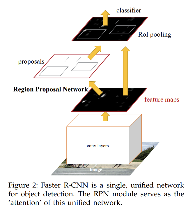
Faster R-CNN은 2가지 모듈로 이루어지며, 첫째는 RPN, 둘째는 RPN의 proposed region을 사용하는 Fast R-CNN detector다. RPN은 Fast R-CNN에게 어딜 볼지 알려주는 attention 역할을 한다.
RPN은 임의의 크기의 이미지를 input으로 받아 각자 objectness score를 가진 set of rectangular object proposals를 output으로 반환한다.
region proposal을 만들기 위해 마지막 shared convolutional layer에 의해 생성된 convolutional feature map output 위로 작은 network를 slide한다. 작은 network는 input convolutional feature map의 n × n spatial window를 input으로 받는다(논문에선 n=3 사용). 각 sliding window는 lower-dimensional feature로 mapping된다. 이 feature은 두 sibling FC layers, 다시 말해 box-regression layer (reg)와 box-classification layer (cls)로 들어간다.
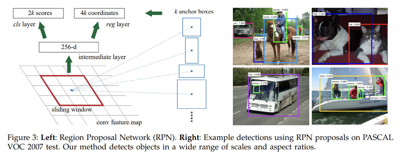
각 sliding-window 위치마다 여러 region proposal를 동시에 예측하며, 가능한 proposal 최대 개수는 k다. 그러므로 reg layer은 k개 box의 좌표를 나타내는 4k outputs을 cls layer은 (softmax로) object인지 아닌지의 확률을 나타내는 2k scores을 계산한다.
k proposals는 k reference boxes에 상대적으로 parameterize되는데, 이 reference box를 anchor이라고 부른다. anchor은 sliding window과 중심을 맞추어 scale과 aspect ratio와 연관된다. 논문에선 default로 3종류 scale과 3종류 aspect ratio로 k=9를 사용한다.
기존의 다른 MultiBox method와 달리 이 모델은 translation invariant한 특징이 있다. 이 특징은 모델 크기도 줄여주고, 따라서 작은 dataset에 overfitting될 가능성도 줄여준다.
이러한 anchor design은 여러 scale과 aspect ratio를 다룰 수 있게 한다. 논문의 pyramid of anchors 방식은 기존의 pyramid of images와 pyramid of filters 방식보다 cost-efficient하다. 여러 scale과 aspect ratio를 가진 anchor boxes를 reference로 bounding box를 regress하고 classify하기 때문이다. 모델은 오직 single scale image와 single scale feature map, single size filter을 쓴다. 그리고 single scale image로 계산한 convolutional feature를 사용하기에 같은 방식의 Fast R-CNN과 호환될 수 있다.
RPN을 학습시키기 위해 각 anchor에 object인지 아닌지의 binary class label를 할당한다. ground-truth box와 IoU overlap이 가장 높은 anchor/anchors와 ground-truth box와 IoU가 0.7보다 높은 anchor, 이 두 종류 anchor에 positive label을 붙여준다. 하나의 ground-truth box가 여러 anchor에 positive label을 붙일 수도 있는 것이다. 두 번째 기준이 positive sample을 하나도 못 찾을 경우를 대비해 첫 번째 기준이 있는 것이다. negative label은 모든 ground-truth box와 IoU가 0.3보다 작은 non-positive anchor에 붙인다. anchor이 positive냐 negative냐는 training objective에 기여하지 않는다.
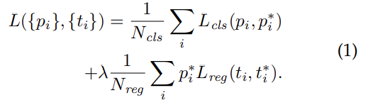
위의 multi-task loss를 최소화한다. i는 mini-batch 내의 anchor의 index, 는 i번째 anchor가 object일지 예측한 probability, 는 anchor이 positive면 1, negative면 0인 ground-truth label, 는 predicted bounding box의 4 parameterized coordinates를 나타내는 vector, 는 positive anchor와 연관된 ground-truth box의 coordinates vector다. cls, reg layer가 각각 , 를 계산한다.
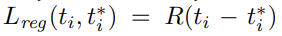
classification loss 는 두 class, 즉 object인지 not object인지에 대한 log loss이다. regressoin loss는 아래와 같으며 R은 robust loss function(=smooth L1)이다. 항에 의해 는 positive anchor에 대해서만 계산된다.
두 항은 , 으로 normalize되고 balancing parameter λ로 조절된다. 논문에선 을 mini-batch size인 256으로 잡았고 을 anchor locations의 (대략적인) 수인 2400으로 잡았다. 실험 결과 λ는 넓은 범위에서 insensitive했다.
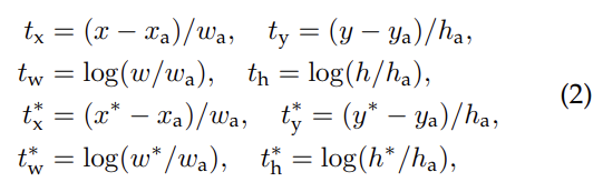
bounding box regression은 위와 같이 사용했다. x, y, w, h는 box의 중심 좌표와 width, height이다. x, , 는 predicted box, anchor box, groundtruth box의 값을 의미한다(y, w, h도 동일). 이는 ground-truth box 근처의 anchor box를 bounding-box로 regression하는 작업으로 볼 수 있다.
RPN training은 back-propagation와 SGD로 end-to-end하게 이루어진다. “image-centric” sampling strategy[2]를 사용해 각 mini-batch는 여러 positive, negative example anchors를 가진 하나의 이미지로부터 얻는다. 모든 anchor의 loss에 대해 optimize하면 dominant한 negative sample에 편향될 것이므로, 대신 이미지에서 256개 anchor을 랜덤하게 sample하여 positive, negative anchor 비율이 거의 1:1이 되게 해서 mini-batch의 loss function을 계산한다. positive sample이 128개 미만이면 mini-batch를 negative들로 pad한다. (즉, 인위적으로 1:1비율이 되게 positive, negative를 뽑는듯)
여기까지가 RPN의 내용이었고 이제 Fast R-CNN과 둘을 합치는 알고리즘에 대해 말해보자. 독립적으로 학습되는 RPN, Fast R-CNN은 convolutional layers를 다르게 변화시킬 것이기 때문에 두 네트워크 간 sharing convolutional layers를 허용하는 기술이 필요하다. 논문은 feature를 공유하는 networks를 학습하는 3가지 방법을 고안했다.
- Alternating training
먼저 RPN을 학습시킨 후, proposal을 사용해 Fast R-CNN을 학습시킨다. Fast R-CNN으로 tune된 network는 다시 RPN을 initialize하는 데 사용된다. 이 과정이 반복된다. 논문의 실험에는 모두 이 방법을 채택했다. - Approximate joint training
- Non-approximate joint training
(2, 3은 생략)
논문은 1번 방법을 선택해 4-Step Alternating Training를 한다. 첫 step에는 RPN을 학습하며, ImageNet-pre-trained model로 초기화되고 region proposal task에 대해 end-to-end로 fine-tuned된다. 두 번째로 step-1 RPN에서 생성된 proposal와 Fast R-CNN을 사용해 separate detection network를 학습한다. 이 detection network도 ImageNet-pre-trained model로 초기화되어 있다. 이 시점에 두 network들은 convolutional layer를 공유하지 않는다. 세 번째로 RPN training을 초기화하기 위해 detector network를 사용한다. 여기서 shared convolutional layers는 고정한 채로 RPN에게 unique한 layers만 fine-tune한다. 이제 두 네트워크가 layer을 공유한다. 마지막으로 shared convolutional layers를 고정한 채로 Fast R-CNN에 unique한 layers를 fine-tune한다. ImageNet pre-trained network로는 ZF net의 “fast” version과 VGG-16, 이렇게 두 종류를 써 봤다.
Strengths
- ablation study를 통해 RPN과 Fast R-CNN detector을 결합한 효과를 입증했다.
- 연산 공유라는 원리를 잘 사용해 속도 향상을 이루었다. Region proposal의 병목을 잘 해결했다.
- 여러 scale input을 넣는 대신 여러 anchor box를 통해 multi-scale invariance를 취득해 계산 효율적이다.
논문에선 RPN이 attention mechanism을 한다고 하는데... 사실 그냥 말만 그런 것 같다.
