Pixel Recurrent Neural Networks

오늘 리뷰할 논문은 autoregressive (AR) model인 PixelCNN & PixelRNN 논문이다. 여러 논문에 몇 번 언급되서 궁금해서 잧아보게 되었다.

아래 포스트를 먼저 보면 도움이 될 것이다.

• Pixel Recurrent Neural Network
• [PR12-Video] 24. Pixel Recurrent Neural Network

---

Summary

natural image의 distribution을 modeling하는 건 비지도학습의 중요한 과제다. 이 과제는 한번에 expressive, tractable, scalable한 image model을 요구한다. 논문은 2차원 이미지 내 픽셀을 순서대로 예측하는 network를 소개한다. 논문의 방법은 raw pixel values의 discrete probability를 모델하고 이미지 내의 complete set of dependencies를 encode한다. fast twodimensional recurrent layers와 deep recurrent network 내의 residual connections이 architecutural novelty다. natural images에 기존 SOTA보다 좋은 log-likelihood scores를 달성한다.

generative modeling의 가장 중요한 난관 중 하나는 complex & expressive하면서 동시에 tractable & scalable한 모델을 만드는 것이다.

논문은 two-dimensional RNNs를 발전시켜 natural images의 large-scale modeling에 적용한다. 결과물인 PixelRNNs은 12개의 fast
two-dimensional Long Short-Term Memory (LSTM) layers로 구성된다. 이 layers은 state에 LSTM을 사용하고, 데이터의 sptial dimensions 중 하나를 따라(along) 모든 states를 한 번에 계산하기 위해 convolution을 사용한다. 이런 layers를 두 종류 개발했다. 첫째는 Row LSTM layer이고, convolution이 각 row를 따라(along) 적용된다. 둘째는 Diagonal BiLSTM layer이고, convolution이 사진의 대각선을 따라(along) 적용된다. 또한 네트워크는 LSTM layers 주변에 residual connections을 포함시킨다. 이는 최대 12층 깊이까지 PixelRNN의 훈련을 도왔다.

또 PixelRNN의 핵심 요소를 공유하며 간략화된 architecture인 PixelCNN을 제안한다. CNN도 Masked convolutions을 사용하면 fixed dependency range을 가진 sequence model로 사용될 수 있다. PixelCNN은 15층으로 이루어진 fully convolutional network이며 layers를 통과하는 동안 input의 spatial resolution를 유지하며 각 location의 conditional distribution을 output한다.

PixelRNN와 PixelCNN은 latent variable models처럼 independence assumptions을 도입하지 않고도 pixel inter-dependencies의 full generality를 포착한다. dependencies는 또한 각 개별 pixel 내의 RGB color values 간에도 유지된다. pixel을 continuous values로 model했던 기존 방식들과 달리 논문은 simple softmax layer로 구현된 multinomial distribution을 사용해 pixel을 discrete value로 모델한다. 이는 모델에 representationl 이점과 training 이점을 모두 제공한다.

논문의 기여는 다음과 같다.

1. 두 종류의 LSTM layers에 상응하는 두 종류의 PixelRNNs을 디자인한다. 가장 빠른 architecture인 purely convolutional PixelCNN을 설명한다. PixelRNN의 Multi-Scale version을 디자인한다.
2. 모델에 discrete softmax distribution을 사용하고 LSTM layers에서 residual connections을 쓰는 선택의 상대적인 장점을 보인다.
3. MNIST와 CIFAR-10에 테스트해서 모델이 SOTA보다 좋은 log-likelihood score을 얻음을 보인다.
4. 32 × 32와 64 × 64 pixels로 resize된 large-scale ImageNet dataset의 결과를 보인다.
5. PixelRNN이 생성한 samples에 정성 평가를 한다.

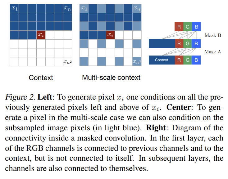
논문의 목표는 natural images의 likelihood를 tractably compute하고 새로운 image를 생성할 수 있는 distribution을 추정하는 것이다. 네트워크는 이미지를 한 번에 한 row씩 스캔하고 각 row 내에서 한 번에 한 pixel씩 스캔한다. 각 pixel에 대해 scanned context가 주어졌을 때 가능한 pixel values에 대한(over) conditional distribution을 예측한다. pixels에 대한(over) joint distribution은 conditional distribution의 곱으로 factorize된다. 예측에 사용되는 parameters는 모든 pixel position에서 공유된다.

• Generating an Image Pixel by Pixel

목표는 n×n pixels로 구성된 각 image x에 probability p(x)를 할당하는 것이다. image x를 1차원 sequence $x_1, ..., x_{n^2}$로 쓸 수 있다. joint distribution p(x)은 conditional distributions의 곱으로 추정된다.

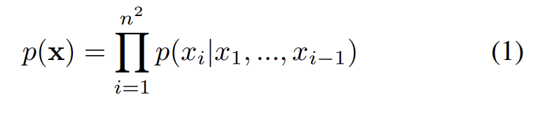
$p(x_i|x_1, ..., x_{i−1})$은 이전 모든 pixels이 주어졌을 때 i번째 pixel x_i의 probability 값이다. generation은 row by row & pixel by pixel로 진행된다.

각 pixel x_i는 RGB channel의 세 값에 의해 공동으로 결정된다.

따라서 각 color은 다른 color와 이전까지의 모든 생성된 pixel에 condition된다. training과 evaluation 중엔 pixel의 distribution이 병렬로 계산되지만 generation 중엔 sequential하다는 것을 주의하라.

기존 방법과 달리 p(x)를 discrete distribution으로 모델하며 식 (2)의 모든 conditional distribution이 softmax layer로 model된 다항식(multinomial)이다. 각 channel variable $x_{i,∗}$은 단순히 256개의 값 중 하나를 가진다. discrete distribution은 representationally simple하고 shape에 prior 없이 arbitrarily multimodal한 장점을 가진다.

• Row LSTM

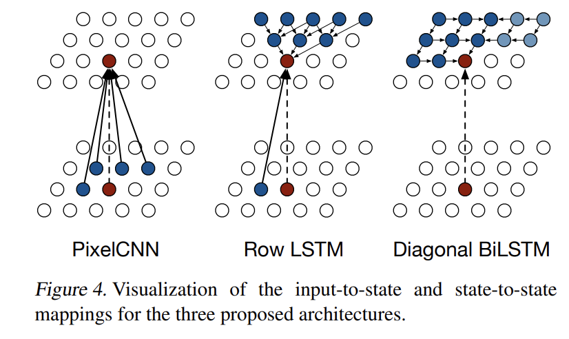
Row LSTM은 unidirectional layer이며 이미지 내의 row를 꼭대기에서 바닥까지 차례대로 한 번에 한 row 전체에 대한 feature를 계산한다. 연산은 one-dimensional convolution로 수행된다. pixel x_i에 대해 layer은 Fig 4처럼 pixel 위의 roughly triangular context을 포착한다. 1차원 convolution의 kernel은 k × 1, k ≥ 3 크기이며 k값이 클수록 포착되는 context가 넓어진다. convolution의 weight sharing은 각 row에 따라 계산되는 features의 translation invariance을 보장한다.

연산은 다음과 같이 진행된다. LSTM layer은 input-to-state component와 recurrent state-to-state component를 가지며 둘을 사용해 LSTM 내의 4 gates를 결정한다. Row LSTM 내의 parallelization을 강화하기 위해 input-to-state component이 먼저 전체 two-dimensional input map에 대해 계산된다. 이때 LSTM 자신의 row-wise orientation를 따르기 위해 k × 1 convolution이 사용된다. convolution은 valid context만 포함하도록 mask되며 (input map 내 각 position에 대한 4 gate vectors를 나타내는) size 4h × n × n의 tensor를 생성한다(h는 output feature maps의 수).

LSTM layer의 state-to-state component의 한 step을 계산하기 위해 각각 h × n × 1 크기의 previous hidden states $h_{i-1}$와 cell states $c_{i−1}$이 주어진다. hidden state와 cell state는 다음과 같이 계산된다.

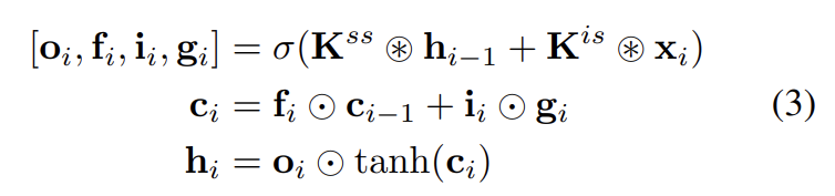
h × n × 1 크기의 x_i는 input map의 row i고 동그라미눈꽃 기호는 convolution operation이고 동그라미점 기호는 element-wise multiplication이다. weights $K^{ss}, K^{is}$는 state-to-state와 input-to-state components의 kernel weights다. 후자는 앞서 설명한 것처럼 precompute된다. output, forget, input gates $o_i, f_i, i_i$의 activation σ는 logistic sigmoid function이고 content gate $g_i$의 σ는 tanh 함수다. 각 step마다 input map의 entire row에 대한 new state를 한번에 계산한다. Row LSTM이 triangular receptive field를 가지기 때문에 entire available contex를 포착하기는 불가능하다.

• Diagonal BiLSTM

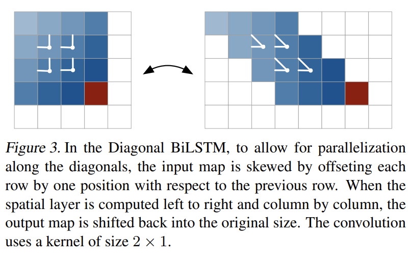
연산을 병렬화하고 임의의 사진 크기에 대해 entire available context를 포착하기 위해 Diagonal BiLSTM을 고안했다. layer의 각 두 방향이 사진을 꼭대기 구석에서 시작해서 대각선 방식으로 scan해서 바닥의 반대쪽 구석에 도착한다. 각 step마다 대각선을 따라 LSTM state을 계산한다.

diagonal computation은 다음과 같이 진행된다. 첫째로 input map을 (대각선을 따라 convolution을 적용하기 쉽게 해주는) space로 왜곡한다(skew). Fig 3처럼 skewing operation은 input map의 각 row를 직전 row에 대한 one position만큼 offset한다. 이는 n × (2n − 1) 크기의 map을 초래한다. 이 시점에서 우리는 Diagonal BiLSTM의 input-to-state와 state-to-state components을 계산할 수 있다. 각 두 방향에 대해 input-to-state component은 LSTM core의 4 gates에 기여하는 단순한 1×1 convolution $K^{is}$이며 연산은 4h × n × n tensor을 생성한다. 그 다음 state-to-state recurrent component이 커널 크기 2 × 1인 column-wise convolution $K^{ss}$를 가지고 계산된다. 이 단계는 previous hidden/cell states를 가지고 input-to-state component의 contribution을 조합해 식 (3)에 따라 next hidden/cell states를 생성한다. output feature map은 offset position을 제거해 다시 n × n map로 복원된다. 이 연산은 각 두 방향에 대해 반복된다. 두 output maps가 주어졌을 때, layer가 future pixel을 보는 걸 방지하기 위해 right output map은 1 row만큼 아래로 shift되서 left output map에 더해진다.

full dependency field을 얻는 것뿐 아니라 Diagonal BiLSTM은 2 × 1 크기의 convolution kernel을 사용해 각 step마다 최소한의 정보를 처리해 highly nonlinear computation을 만든다는 장점이 있다. 2 × 1보다 큰 kernel size는 (이미 global한 receptive field를 더 넓히지 못하기 때문에) 딱히 유용하지 않다.

• Residual Connections

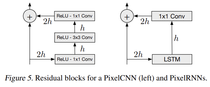
PixelRNN을 12층 깊이까지 학습시킨다. 수렴 속도를 증가시키고 network를 통해 더 직접적으로 신호를 전파하기 위해 residual connection을 배치했다.

PixelRNN LSTM layer로의 input map은 2h features를 가진다. input-to-state component은 gate 당 h features을 생산하여 features의 수를 줄인다. recurrent layer을 적용한 후, 1 × 1 convolution을 통해 output map은 다시 position 당 2h features로 upsample되고 input map이 output map에 더해진다. residual connection과 별개로 각 layer에서 output으로 learnable skip connections을 사용할 수도 있으며, 이후 실험에서 residual connection과 layer-to-output skip connections의 효과를 비교한다.

• Masked Convolution

모든 layer에서 각 input position에 대한 h features은 세 부분으로 분할되는데, 각각 RGB channel의 하나에 상응한다. 현재 pixel x_i에 대한 R channel을 예측할 때는 왼쪽과 위의 generated pixels만 context로 사용될 수 있다. G channel을 예측할 때는 previously generated pixels에 R channel의 값까지 context로 사용될 수 있고 마찬가지로 B channel을 예측할 때는 R과 G까지도 사용할 수 있다. 이 dependencies에 대한 connection을 제한하기 위해 PixelRNN 내의 inputto-state convolutions와 다른 purely convolutional layers에 mask를 적용한다.

Fig 2와 같이 mask A, mask B라고 이름붙인 두 종류 mask를 사용한다. mask A는 PixelRNN의 first convolutional layer에만 적용되며 neighboring pixels와 현재 pixels 내의 이미 예측된 colors로의 connections을 제한한다. 반면 mask B는 모든 subsequent input-to-state convolutional transitions에 적용되어 color에서 자기자신으로의 연결을 허용함으로써 mask A의 제한을 완화한다. 각 update 후의 input-to-state convolutions 내의 상응하는 weights을 0으로 만드는 방식으로 masks는 쉽게 구현될 수 있다.

• PixelCNN

Row/Diagonal LSTM layers은 그들의 receptive field 내에서 잠재적으로 unbounded dependency range을 가진다. 각 states가 순차적으로 계산되어야 하기 때문에 이는 computational cost가 된다. 하나의 대안책은 receptive field를 크지만 unbounded하지 않게 만드는 것이다. standard convolutional layers를 사용해 bounded receptive field를 포착하고 모든 pixel positions에 대한 feature을 한번에 계산할 수 있다. PixelCNN은 spatial resolution을 보존하는 multiple convolutional layers을 사용하며 pooling layers은 사용되지 않는다. future context를 보는 걸 막기 위해 convolution에 mask가 적용된다. PixelRNN에 비한(over) PixelCNN의 장점인 병렬화는 training/evaluating에만 가능하다는 것에 주의하라. image generation process은 두 모델 모두 sequential하다.

• Multi-Scale PixelRNN

Multi-Scale PixelRNN은 unconditional PixelRNN와 하나 이상의 conditional PixelRNNs으로 구성된다. 먼저 unconditional PixelRNN이 original image에서 (일반적인 방법으로) smaller s×s image을 subsample한다. 그 다음 conditional PixelRNN이 s × s
image를 추가적인 input으로 받아서 Fig 2처럼 larger n × n image을 생성한다.

conditional network는 standard PixelRNN과 비슷하지만 각 layer이 small s × s image의 upsampled version으로 편향되어 있다. upsampling과 biasing은 다음과 같이 정의되어있다. upsampling의 경우 c × n × n 크기의 enlarged feature map을 구성하기 위해 deconvolutional layers을 가진 convolutional network을 사용한다(c는 upsampling network의 output map 내 features의 수). 그 다음 biasing process에선 conditional PixelRNN 내의 각 layer에 대해 단순히 c × n × n conditioning map을 4h × n × n map으로 map하고 이를 상응하는 layer의 input-to-state map에 더한다. 이는 1 × 1 unmasked convolution으로 수행된다. 그다음 일반적인 방식으로 larger n × n image이 생성된다.

네트워크는 4종류를 만들었다. Row LSTM 기반 PixelRNN, Diagonal BiLSTM 기반 PixelRNN, fully convolutional (=PixelCNN)과 MultiScale PixelRNN이다.

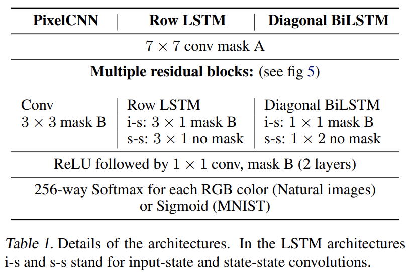
Tab 1은 single-scale networks 내의 각 layer을 명시한다. first layer은 mask A를 쓰는 7 × 7 convolution이다. 그 다음 두 종류의 LSTM networks이 여러(variable number) recurrent layers를 사용한다. 이 layer의 input-to-state convolution은 mask B를 쓰는 반면 state-to-state convolution은 mask되지 않는다. PixelCNN은 mask B를 가지고 3 × 3 convolution을 사용한다. 그 다음 top feature map이 ReLU와 1×1 convolution를 포함하는 여러 layers를 통과한다. CIFAR-10와 ImageNet 실험의 경우 이 layers은 1024 feature maps를 가진다. MNIST 실험은 32 feature maps를 가진다. 세 네트워크 모두 layers 사이 Residual/layer-to-output connections이 사용된다.

모든 모델은 discrete distribution에서 온 log-likelihood loss function으로 학습되고 평가된다. natural image data는 주로 continuous distribution으로 model되지만 다음과 같은 방법으로 우리 방식을 기존 방식과 비교할 수 있다. (생략)

실험 결과는 생략하고 흥미로운 일부만 설명하겠다.

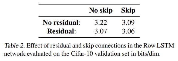
residual connection과 skip connection 모두 도움이 되었다. 둘 다 사용했을 때는 12층까지 깊이가 증가할수록 Row LSTM의 성능이 향상됐다.

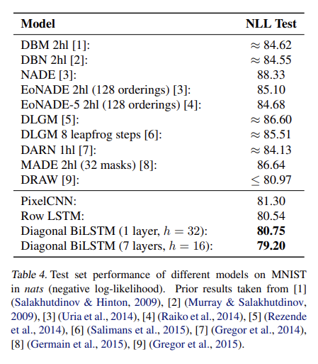
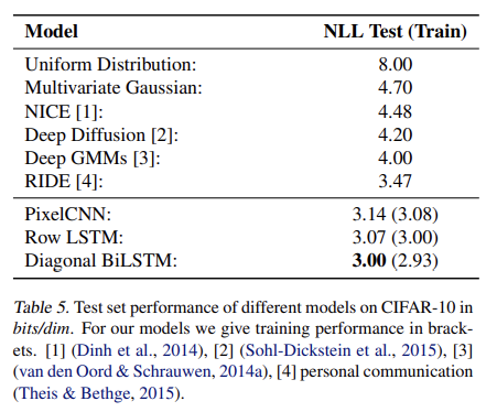
CIFAR-10 데이터셋의 경우 Diagonal BiLSTM 성능이 가장 좋았고 Row LSTM과 PixelCNN이 뒤따랐다. 이는 receptive field 때문인데, Diagonal BiLSTM은 global view를 가지고 Row LSTM은 partially occluded view을 가지고 PixelCNN은 context에서 가장 적은 pixel을 보기 때문이다.

Strengths

1. RNN을 써서(엄밀히는 LSTM) generative model을 만든 게 흥미로웠다. context를 state에 저장해서 receptive field 역할을 한 것 같다.
2. 기존 방식과 달리 softmax layer을 써서 픽셀 값을 discrete한 관점으로 보았다.