Neural Turing Machines

오늘 리뷰할 논문은 구글 딥마인드의 NTM 논문이다.

아래 포스트를 먼저 보면 도움이 될 것이다.

• Neural Turing Machines 리뷰
• Neural Turing Machines
• NTM(Neural-Turing-Machine) 코드 리뷰

---

neural network에 external memory resource를 달아줘서 attentional process로 상호작용할 수 있게 했다. 시스템은 Turing Machine이나 Von Neumann architecture와 비슷하지만 end-to-end로 미분가능하기 때문에 gradient descent로 학습될 수 있다. NTM은 copying, sorting, associative recall 같은 간단한 알고리즘을 추론할 수 있다.

컴퓨터 프로그램은 elementary operations (e.g., arithmetic operations), logical flow control (branching), external memory의 세 가지 근본적인 메커니즘을 사용한다. 그러나 머신러닝은 logical flow control와 external memory의 사용을 무시해왔다.

한편 RNNs은 Turing-Complete고 임의의 함수(procedure)를 simulate할 능력이 있지만 실제로 그러기는 쉽지 않았다. 논문은 large, addressable memory를 통해 “Neural Turing Machine” (NTM)을 만들고 program을 학습하는 practical mechanism을 보인다.

human cognition에서 algorithmic operation와 가장 비슷한 process는 working memory다. working memory란 정보의 short-term storage과 rule-based manipulation 능력을 의미한다. computational 측면에서 이 rules는 간단한 프로그램이며, 저장된 정보가 이 프로그램들의 매개변수(arguments)가 된다. 따라서 NTM은 working memory를 닮았고, “rapidly-created variables”와 비슷한(approximate) rules의 응용(application)을 필요로 하는 tasks를 해결하기 위해 디자인되었다. Rapidly-created variables는 (register에서 숫자 3과 4가 저장되어 7로 더해지는 것처럼) memory slots에 빠르게 묶인(quickly bound) 데이터를 의미한다. 또 NTM은 attentional process를 통해 메모리를 선택적으로 읽거나 쓸 수 있다는 점에서도 working memory와 비슷하다. 대부분의 working memory 모델과 달리 NTM은 symbolic data에 대한 fixed set of procedures를 배포하는 게 아니라 (즉 함수가 고정된 게 아니라) working memory를 사용하는 법을 학습한다.

(기존 연구 설명 흥미로운데 길어서 생략)

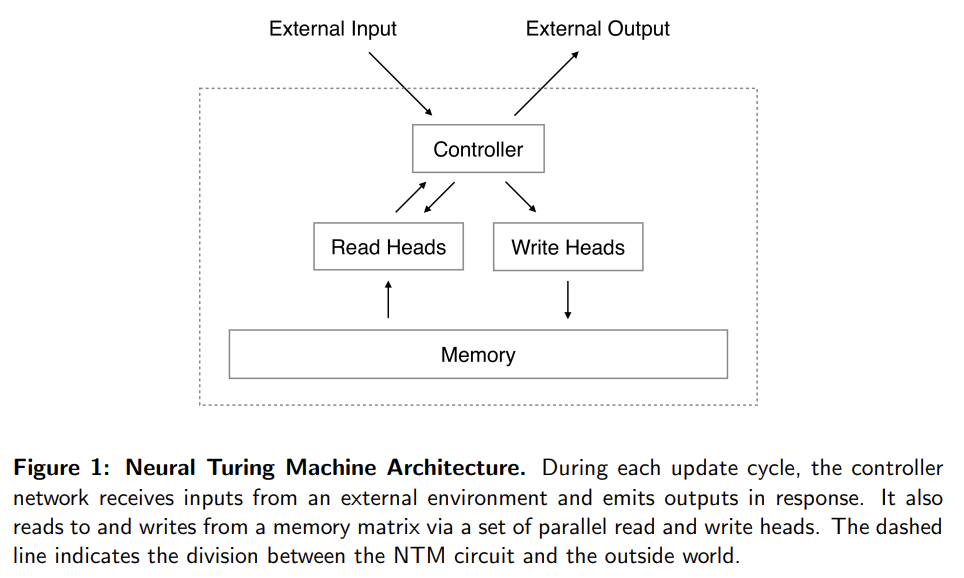
NTM은 두 기본 요소로 이루어진다. neural network controller와 memory bank다. controller는 일반적인 neural network처럼 input/output vector를 통해 외부 세계와 상호작용한다. 그러나 일반적인 네트워크와 달리 selective read/write operation을 통해 memory matrix와도 상호작용한다. Turing machine에 비유해 이 operations을 parameterise하는 network outputs를 'heads'라고 부른다.

NTM의 모든 구성요소는 미분가능해서 gradient descent로 학습할 수 있다. 이는 (single element에 addressing하는 일반적인 Turing machine이나 컴퓨터와 달리) ‘blurry’ read/write operations를 사용해 memory 내 모든 element에 greater/lesser degree로 상호작용한다. degree of blurriness는 attentional “focus” mechanism로 결정된다. attentional “focus” mechanism은 각 read/write operation이 memory의 작은 부분과 상호작용하고 나머지는 무시하게 제약한다. memory와의 상호작용이 몹시 드물기(sparse) 때문에 NTM은 inference 없이 data를 저장(sotre)하는 데 편향되어 있다. attentional focus을 받은(bring into) memory location은 head로 덩든 specialised outputs로 결정된다. 이 outputs는 memory matrix 내의 rows에 대한(=memory location) normalised weighting을 정의한다. (read/write head 당 하나의) 각 weighting은 각 location에서 head가 read/write하는 정도를 정의한다. 따라서 head는 single location에 sharply attend할 수도 있고 많은 location에 weakly attend할 수도 있다.

• Reading

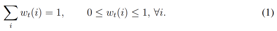
$M_t$가 time t에서 N × M memory matrix의 contents, N이 memory locations의 수, M이 각 location에서 vector size라고 두자. $w_t$는 time t에 read head로 구한, N locations에 대한 weighting vector라고 두자. 모든 가중치가 정규화되어있으므로 $w_t$의 N elements wt(i)는 다음 제약을 만족한다.

head가 반환한 length M read vector $r_t$는 메모리 내의 row-vectors $M_t(i)$의 convex combination으로 정의된다.

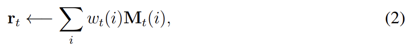
이는 memory와 weighting 둘 모두에 미분가능하다.

• Writing

LSTM의 input/forget gates에서 영감을 받아 각 write를 두 부분으로 분해한다. 바로 erase와 뒤따르는 add이다.

time t에 write head로부터 weighting $w_t$가 (M elements가 모두 (0,1) 범위에 있는) erase vector $e_t$와 함께 주어졌을 때 직전 time step의 memory vectors $M_{t−1}(i)$는 다음과 같이 수정된다.

(대괄호는 index가 아니라 단순히 곱하기)

1은 요소가 전부 1인 row-vector고 memory location에 대한 multiplication은 point-wise로 수행된다. 따라서 memory location의 elements는 그 location에의 weighting과 erase element가 1일 때만 0으로 reset된다. weigting이나 erase 어느 한쪽이라도 0이면 memory는 변하지 않는다. write head가 여러 개 존재하면 (곱연산 교환법칙이 성립하기 때문에) erasures는 아무 순서로 수행되도 된다.

각 write head는 또한 length M add vector $a_t$를 생산하며 이는 erase step 후에 memory에 더해진다.

마찬가지로 heads가 여럿일 때 adds의 수행 순서도 상관없다. 모든 write heads의 combined erase & add operations가 시간 t에 memory의 최종 content를 생성한다. erase와 write가 모두 미분가능하므로 composite write operation도 미분가능하다. erase와 add vectors는 M independent components를 가지며 각 memory location에서 어떤 element가 수정될지 fine-grained control을 허용한다.

• Addressing Mechanisms

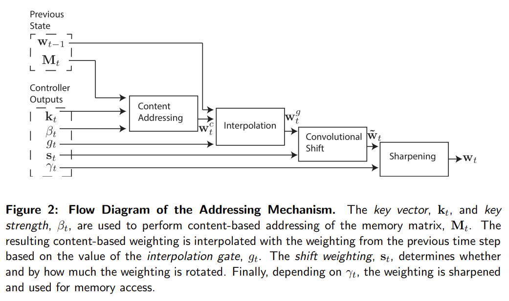
그럼 weighting은 어떻게 만들까? weigting은 complementary facilities를 가진 두 addressing mechanism을 조합해 구한다. 첫번째 메커니즘인 “content-based addressing”은 current values와 controller로 얻은 values 간 유사도에 기반한 locations에 attention을 집중한다.

하지만 모든 문제가 content-based addressing으로 풀리는 건 아니다. 일부 tasks에선 variable의 content가 arbitrary하지만 variable이 여전히 인식할 수 있는 이름이나 주소가 필요하다. arithmetic problems가 이런 종류인데, 예를 들어 변수 x와 y는 어느 값이든 취할 수 있지만 함수 f(x, y) = x × y는 여전히 정의되야 한다. 이런 task를 위한 controller는 x와 y의 값을 받아 서로 다른 주소에 저장한 후 그들을 retrieve해 곱하기 알고리즘을 수행할 수 있다. 이 경우 변수들은 content가 아니라 location으로 address된다. Content-based addressing는 그 memory location의 content에 location 정보를 저장할 수 있기 때문에 엄밀히 말하면 location-based addressing보다 일반적이다. 그러나 실험해 보니 location-based addressing를 primitive operation으로 제공하는 것은 몇몇 형태의 generalisation에 필수적임이 드러나서 두 mechanism을 동시에 채택했다.

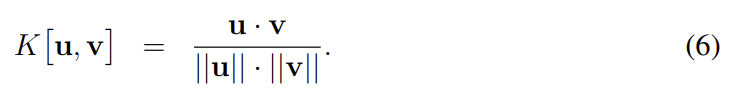
content-addressing의 경우, (read든 write든) 각 head는 우선 length M key vector $k_t$를 생성한다. 이는 similarity measure K[,]로 각 vector $M_t(i)$와 비교된다. content-based system은 similarity와 (focus의 precision을 증폭하거나 희석시키는) positive key strength $β_t$에 기반해 normalised weighting $w^c_t$를 생성한다.

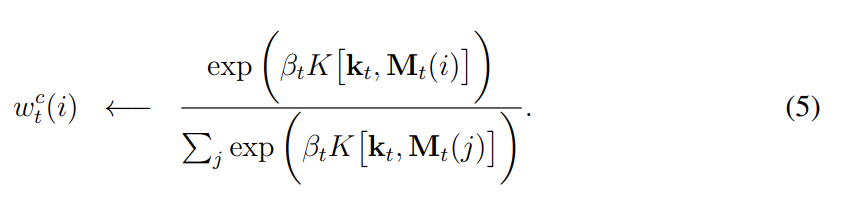
실험에서 similarity measure K는 cosine similarity를 사용했다.

location-based addressing mechanism는 memory location에 걸친 simple iteration과 random-access jumps가 모두 가능하도록 디자인되었다. 이는 weighting의 rotational shift를 통해 구현되었다. 예를 들어 현재 weighting이 전적으로 single location에 focus한다면, 1만큼의 rotation은 focus를 다음 location으로 옮길 것이다. negative shift는 반대 방향으로 옮길 것이다.

rotation에 앞서 각 head는 (0, 1) 범위의 스칼라 interpolation gate $g_t$를 구한다. g의 값은 직전 time step에서 head가 생성한 weighting $w_{t-1}$과 현재 time step에서 content system이 생성한 weighting $w^c_t$ 사이를 blend해서 gated weighting $w^g_t$를 만든다.

gate가 0이면 content weighting가 완전히 무시되며 직전 time step으로부터의 weighting이 사용된다. 역으로 gate가 1이면 직전 time step의 weighting이 무시되고 content-based addressing만 적용된다.

interpolation 이후 각 head는 shift weighting $s_t$를 얻고 이는 allowed integer shifts에 대한 normalized distribution을 정의한다. 예를 들어 만약 -1에서 1 사이 shift가 허용된다면 $s_t$는 -1, 0, 1의 shift에 해당하는 세 element를 가진다. shift weightings를 정의하는 가장 간단한 방법은 올바른 크기의 softmax layer를 controller에 부착해 사용하는 것이다.

0~N-1의 N memory locations를 index한다면, $s_t$로 $w^g_t$에 적용한 rotation은 다음 circular convolution로 표현될 수 있다.

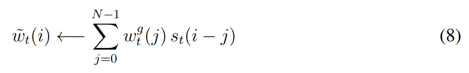
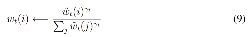
모든 index arithmetic은 modulo N으로 연산되었다. 식 (8) 내의 convolution operation은 (shift weighting이 sharp하지 않다면) 시간이 지남에 따라 weightings의 leakage나 dispersion를 초래할 수 있다. 예를 들어 -1, 0, 1의 shift가 0.1, 0.8, 0.1의 weight으로 주어질 때 rotation은 single point에 집중된 weighting을 세 points에 slightly blurred된 weighting으로 바꿔놓을 것이다. 이를 해결하기 위해 각 head는 하나의 추가적인 scalar $γ_t ≥ 1$를 얻어 final weighting을 다음과 같이 sharpen한다.

weighting interpolation과 content/location-based addressing의 combined addressing system은 세 가지 complementary modes로 작동할 수 있다. 첫째로 weighting이 location system에 의한 수정 없이 content system로 정해질 수 있다. 둘째로 content addressing system로 생성된 weighting이 선택되어 shift될 수 있다. 이는 content로 접근한 주소 옆의 location으로 focus를 점프시킬 수 있다. computational 측면에서 이는 head가 contiguous block of data를 찾아 그 block 내의 특정 element에 접근하는 것을 가능하게 한다. 셋째로, 이전 time step에서의 weighting이 content-based addressing system에서 아무런 input도 없이 rotate될 수 있다. 이는 각 time step에서 동일한 거리를 이동함으로써(advancing) weighting이 sequence of addresses를 iterate할 수 있게 한다.

• Controller Network

앞서 설명한 NTM architecture은 memory 크기, read/write heads의 수, allowed location shifts의 범위 등의 hyperparameter가 있다. 그러나 가장 중요한 architectural choice는 controller로 사용할 neural network의 종류다. 구체적으로 recurrent network를 쓸 건지 feedforward network를 쓸 건지가 중요하다. LSTM 같은 recurent controller는 matrix의 larger memory를 보완할 수 있는 고유의 internal memory가 있다. 이는 controller가 operation의 여러 time steps에 걸친 정보를 조합할 수 있게 한다. 반면 feedforward controller는 모든 step에서 memory 내의 동일한 location을 읽고 쓰는 것으로 recurrent network를 모방할 수 있다. 또한 feedforward controllers는 네트워크의 operation에 자주 greater transparency를 부여하는데, memory matrix에 읽고 쓰는 패턴은 보통 RNN의 internal state보다 해석하기 쉽기 때문이다. 그러나 feedforward network의 단점은 동시에 사용하는 read/write heads의 숫자가 NTM이 수행하는 연산의 종류에 병목을 부과한다는 것이다. single read head로는 각 time step에 single memory vector에 unary transform만 수행할 수 있고 two read heads는 binary vector transforms만 가능하고... 같은 식이다. Recurrent controllers는 이전 time steps에서의 read vectors를 내부적으로 저장할 수 있어 이 문제를 겪지 않는다.

이제 실험은 copying, sorting data sequences 같은 간단한 algorithmic tasks에 수행한다. 목표는 NTM이 그 문제를 풀 수 있다는 것을 보이는 것뿐 아니라, compact internal programs를 학습함으로써 그것이 가능하다는 것을 보이는 것이다. 모든 실험에서 세 종류 architecture, feedforward controller를 가진 NTM, LSTM controller를 가진 NTM, standard LSTM network를 가지고 실험했다. 모든 task가 episodic하기 때문에 각 input sequence의 시작마다 네트워크의 dynamic state를 reset한다. LSTM networks에 대해 이는 previous hidden state를 learned bias vector와 동일하게 세팅한다는 것을 의미한다. NTM에 대해서는 controller의 previous state, previous read vectors의 value, memory의 contents가 모두 bias value로 설정된다. 모든 tasks는 binary targets를 가진 supervised learning problems이다. 모든 네트워크는 logistic sigmoid output layers를 가지고 cross-entropy objective function으로 학습된다.

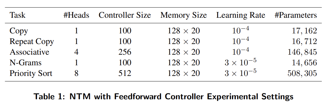
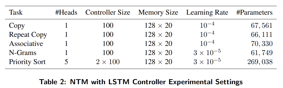
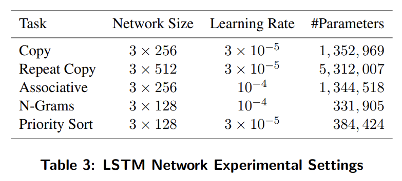
task는 Copy, Repeat Copy, Associative recall, Dynamic N-Grams (N개의 이전 bit에서 다음 bit 예측), Priority Sort에 대해 실험했다. 설명은 생략한다.

Strength

1. 메모리를 사용해 알고리즘을 수행할 수 있는 튜링 머신 개념에 neural network controller를 합쳐 지도학습으로 알고리즘을 학습할 수 있게 했다.
2. 모든 구성요소가 미분가능이라 경사하강법을 사용해 end-to-end로 학습이 가능하다.
3. parameter 수가 LSTM보다 훨씬 적은데 성능은 NTM이 더 좋으니 의도한 대로 메모리를 잘 사용하고 있는 것 같다.

Weaknesses

1. NTM으로 실험한 결과가 완벽하지는 않았다. 일반화 정도에 한계가 있었다.