Auto-Encoding Variational Bayes

오늘 리뷰할 논문은 유명한 VAE 논문이다.

수학이 많고 어려워서 이해도가 낮다.

아래 포스트를 먼저 보면 도움이 될 것이다.

• VAE
• [논문 Summary] VAE (2014 ICLR) "Auto-Encoding Variational Bayes"
• [논문리뷰] VAE(Auto-Encoding Variational Bayes)
• Autoencoder based Anomaly Detection
• posterior과 bayesian

---

Summary

continuous latent variables and/or parameters가 intractable posterior distributions를 가지는 directed probabilistic models로 어떻게 efficient approximate inference and learning을 수행할 수 있나? variational Bayesian (VB) approach은 intractable posterior로의 approximation의 optimization을 포함한다. 그러나 common mean-field approach는 (일반적인 경우에는 역시 intractable한) approximate posterior에 관한 기댓값의 analytical solutions을 요구한다는 문제가 있다.

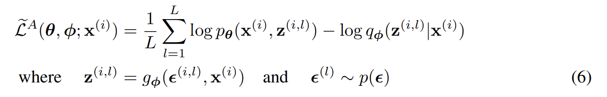
논문은 reparameterization of the variational lower bound가 어떻게 lower bound의 simple differentiable unbiased estimator를 만들 수 있는지 보인다. 이 SGVB (Stochastic Gradient Variational Bayes) estimator는 continuous latent variables and/or
parameters를 가진 거의 모든 모델에서 efficient approximate posterior inference로 사용될 수 있으며 standard stochastic gradient ascent techniques를 사용해 쉽게 optimize할 수 있다.

i.i.d. (independent identically distributed) dataset과 continuous latent variables per datapoint인 경우를 위해 논문은 AutoEncoding VB (AEVB) algorithm을 제안한다. AEVB 알고리즘은 (simple ancestral sampling을 사용해 효율적인 approximate posterior inference를 가능하게 하는) recognition model을 optimize하기 위해 SGVB estimator를 사용함으로써 inference와 learning을 효율적으로 만든다. 이는 MCMC 같은 expensive iterative inference schemes per datapoint 없이도 model parameters를 효과적으로 학습할 수 있게 한다. 또한 learned approximate posterior inference mode는 recognition, denoising, representation, visualization purposes 같은 task에 사용될 수 있다. neural network가 recognition model를 위해 사용될 때 variational auto-encoder가 된다.

이제 lower bound estimator (stochastic objective function)를 고안해보자. 문제 상황을 i.i.d. dataset with latent variables per datapoint를 가지고 (global) parameters에 maximum likelihood (ML) or maximum a posteriori (MAP) inference를, latent variables에 variational inference를 수행하려는 일반적인 경우로 한정하겠다.

• Problem scenario

문제 상황은 다음과 같다. continuous/discrete variable x의 N개 i.i.d. samples을 가지는 dataset $X = \{x^{(i)}\}^N_{i=1}$를 생각해보자. data는 unobserved continuous random variable z와 관련해 어떤 random process로 생성되었다고 가정하자. process는 두 단계로 이루어진다. 1. value $z^{(i)}$가 어떤 prior distribution $p_{θ^∗}(z)$에서 생성되고 2. value $x^{(i)}$ 어떤 conditional distribution $p_{θ^∗}(x|z)$에서 생성된다. prior $p_{θ^∗}(z)$와 likelihood $p_{θ^∗}(x|z)$는 distributions $p_θ(z)$와 $p_θ(x|z)$의 parametric families에서 온다고 가정하고 그들의 PDF(parametric distribution families?)는 θ와 z에 대해 거의 모든 것에서 미분 가능하다고 가정하자. 문제는 프로세스의 많은 부분이 우리에게 숨겨져있다는 것인데, 우리는 true parameters $θ^*$와 values of the latent variables $z^{(i)}$를 모른다.

중요한 점은 marginal or posterior probabilities에 대한 common simplifying assumptions를 하지 않을 것이란 점이다. 논문은 다음 상황에서조차 효과적으로 작동하는 일반적인 알고리즘에 관심을 가진다.

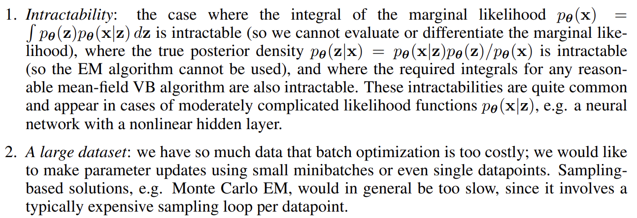
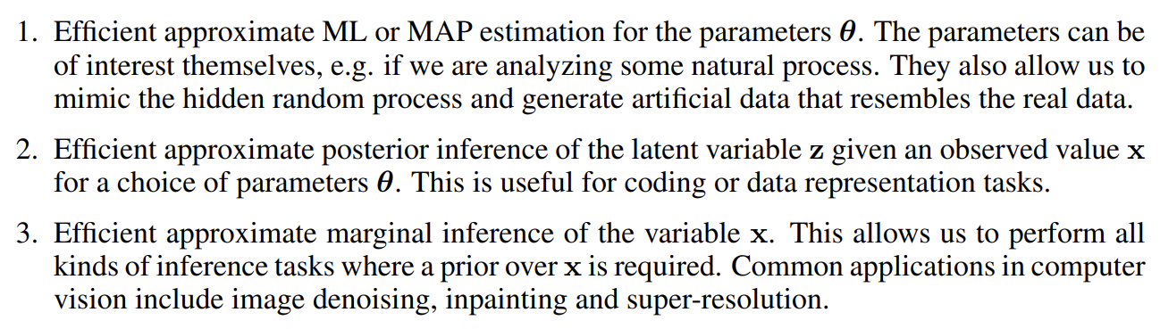
논문은 위 시나리오와 관련해 다음 세 가지 문제에 관심을 가지고 해결책을 제시한다.

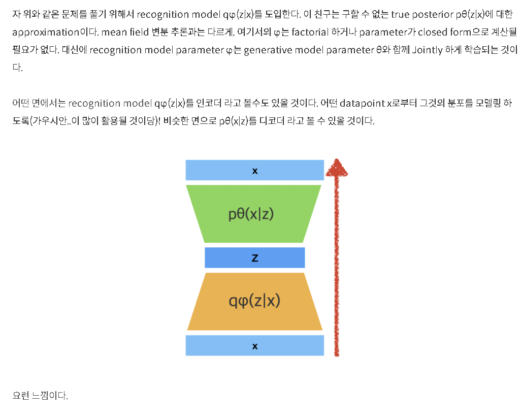
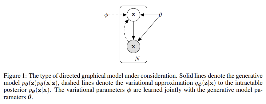
위 문제들을 해결하기 위해 논문은 intractable true posterior $p_θ(z|x)$의 approximation인 recognition model $q_φ(z|x)$을 소개한다. mean-field variational inference에의 approximate posterior와 달리 필수적으로 factorial이 아니며 parameters φ가 어떤 closed-form expectation에서 계산된 게 아님에 주의하라. 대신 recognition model parameters φ를 generative model parameters θ와 공동으로 학습하는 방법을 소개할 것이다.

coding theory perspective에선 unobserved variables z가 latent representation이나 code로 해석될 수 있다. 따라서 논문은 recognition model $q_φ(z|x)$을 probabilistic encoder로도 간주한다. datapoint x가 주어질 때 (x가 생성될 수 있는,) possible values of code z에 대해(over) distribution (e.g. a Gaussian)을 산출하기 때문이다. 비슷하게 true posterior $p_θ(z|x)$을 probabilistic decoder로 간주한다. code z가 주어졌을 때 possible corresponding values of x에 대해(over) distribution을 산출하기 때문이다.

• The variational bound

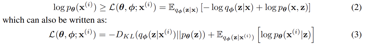
marginal likelihood는 marginal likelihoods of individual datapoints의 합으로 구성된다.

첫 RHS term은 true posterior에서 온 approximate의 KL divergence이다. KL-divergence이 non-negative이기 때문에 두번째 RHS term $L(θ, φ; x^{(i)})$은 marginal likelihood of datapoint i에의 (variational) lower bound라고 불리며 다음과 같이 쓸 수 있다.

우리는 variational parameters φ와 generative parameters θ 모두에 대해 lower bound $L(θ, φ; x^{(i)})$를 미분하고 최적화하고 싶다. 그러나 φ에 대한 lower bound의 gradient는 문제가 있다. 이런 류의 문제에 대한 usual (na¨ıve) Monte Carlo gradient estimator은 $z^{(l)} ∼ q_φ(z|x^{(i)})$일 때 $∇_φE_{q_φ(z)}[f(z)] = E_{q_φ(z)}[f(z)∇_{q_φ(z)}\log q_φ(z)] \simeq {1 \over L} \Sigma^L_{l=1} f(z)∇_{q_φ(z^{(l)})} \log q_φ(z^{(l)})$ 이다. 이 gradient estimator은 아주 높은 variance를 보여서 우리의 목적에는 impractical하다.

• The SGVB estimator and AEVB algorithm

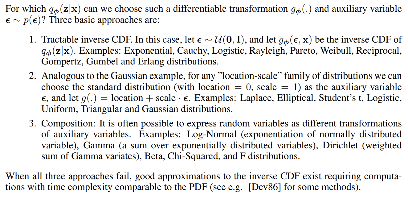
그래서 논문은 lower bound의 practical estimator와 parameter에 대한 estimator의 도함수를 소개한다. 위에서 말한 특정 mild conditions 아래 differentiable transformation $gφ(\epsilon, x)$ of (auxiliary) noise variable $\epsilon$를 사용해 random variable $\tilde z ∼ q_φ(z|x)$를 reparameterize할 수 있다.

이제 $q_φ(z|x)$에 관한 어떤 function f(z)의 기댓값의 Monte Carlo estimates를 다음과 같이 추정할 수 있다.

이를 variational lower bound (식 (2))에 적용해서 generic Stochastic Gradient Variational Bayes (SGVB) estimator $\tilde L^A(θ, φ; x^{(i)}) \simeq L(θ, φ; x^{(i)})$를 얻는다.

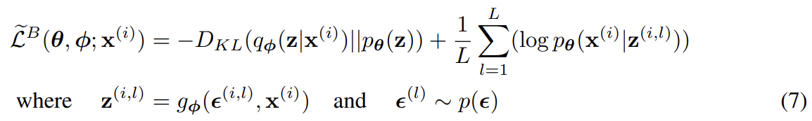
흔히 식 (3)의 KL-divergence $D_{KL}(q_φ(z|x^{(i)})||p_θ(z))$는 analytically 통합될 수 있는데(appendix B), 그런 조건 하에서(such that) 오직 expected reconstruction error $E_{q_φ(z|x^{(i)})} [\log p_θ(x^{(i)}|z)]$만이 sampling을 통한 estimation을 필요로 한다. 그러면 KL-divergence term은 φ를 regularize하여 approximate posterior가 prior $p_θ(z)$와 가깝도록 격려하는 것으로 해석될 수 있다. 이는 식 (3)과 상응해 SGVB estimator $\tilde L^B(θ, φ; x^{(i)}) \simeq L(θ, φ; x^{(i)})$의 두 번째 버전을 만들며, 이는 보통 generic estimator보다 variance가 적다.

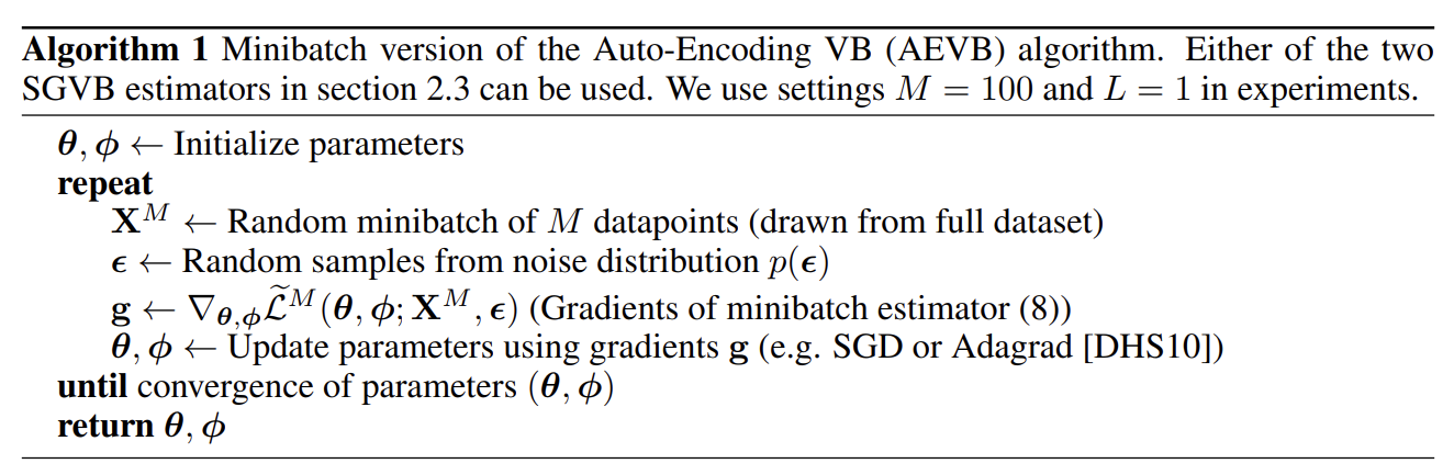
N개의 datapoint를 가진 dataset X에서 복수의 datapoints가 주어졌을 때 minibatch에 기반해 전체 dataset에 대한 marginal likelihood lower bound의 estimator을 다음과 같이 구성할 수 있다.

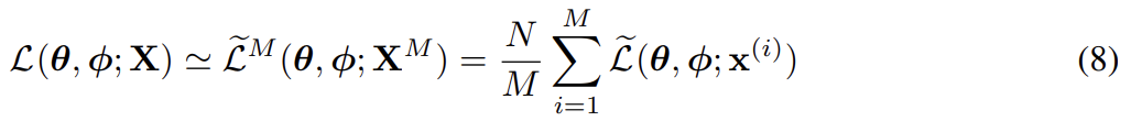
이때 minibatch $X^M = \{x^{(i)}\}^M_{i=1}$은 full dataset X에서 랜덤하게 M datapoints를 sample한 것이다. 실험을 통해 minibatch size M이 충분히 크다면 number of samples L per datapoint를 1로 설정해도 된다는 것을 발견했다. Derivatives $∇_{θ,φ}\tilde L(θ; X^M)$가 구해질 수 있으며 결과 gradients는 SGD나 Adagrad 같은 stochastic optimization methods와 함께 사용될 수 있다. algorithm 1이 stochastic gradients를 계산하는 basic approach를 보여준다.

식 (7)의 objective function을 보면 auto-encoder과의 연관성은 더욱 명확해진다. 첫째 항 (prior에서 온 approximate posterior의 KL divergence)은 regularizer로 작동하고 둘째 항은 expected negative reconstruction error이다. function $g_φ(.)$는 datapoint $x^{(i)}$와 random noise vector $\epsilon^{(l)}$를 그 datapoint에 대한 approximate posterior에서 온 sample로 map하도록 선택된다($z^{(i,l)} = g_φ(\epsilon^{(l)}, x^{(i)}) where z^{(i,l)} ∼ q_φ(z|x^{(i)})$). 그 다음 sample $z^{(i,l)}$는 함수 $\log p_θ(x^{(i)}|z^{(i,l)})$로 넣어지는데, 이는 generative model에서 datapoint $x^{(i)}$의 probability density (or mass)와 동일하다. 이 항은 auto-encoder 관점(parlance)에서 negative reconstruction error이다.

• The reparameterization trick

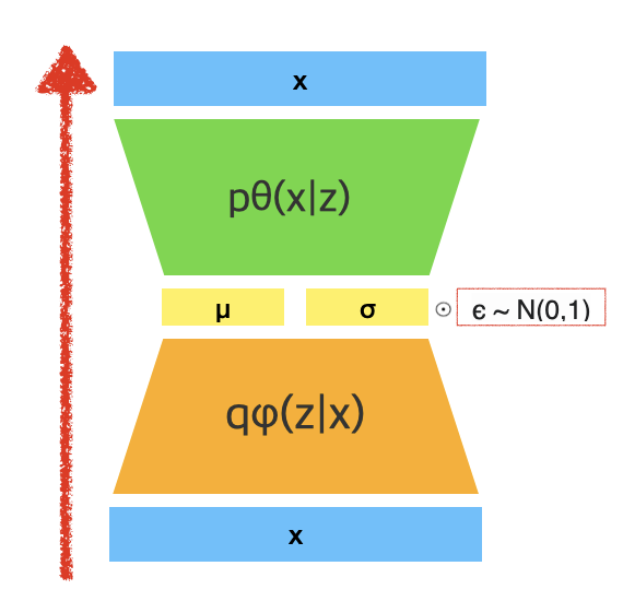
문제를 해결하기 위해 우리는 samples을 $q_φ(z|x)$에서 생성하는 alternative method를 소개했다. essential parameterization trick은 간단한데, z가 continuous random variable이고 $z ∼ q_φ(z|x)$가 어떤 conditional distribution이라 두자. 그러면 random variable z를 deterministic variable $z = g_φ(\epsilon, x)$로 표현할 수 있다. ε은 independent marginal p(ε)를 가진 auxiliary variable이고 $g_φ(.)$은 φ로 parameterized된 어떤 vector-valued function이다.

이 reparameterization은 우리의 경우에 유용한데, 왜냐하면 $q_φ(z|x)$에 관한 expectation이 Monte Carlo estimate이 φ에 대해 미분가능해서 expectation을 rewrite하는 데 사용될 수 있기 때문이다. 증명은 다음과 같다. deterministic mapping $z = g_φ(\epsilon, x)$이 주어졌을 때 우리는 $q_φ(z|x) \Pi_i dz_i = p(\epsilon) \Pi_i d\epsilon_i$인 것을 안다. 따라서 $\int q_φ(z|x)f(z) dz = \int p(\epsilon)f(z) d\epsilon = \int p(\epsilon)f(g_φ(\epsilon, x)) d\epsilon$가 된다. $\epsilon^{(l)} ∼ p(\epsilon)$일 때 differentiable estimator가 $\int q_φ(z|x)f(z) dz \simeq {1 \over L} \Sigma^L_{l=1} f(g_φ(x, \epsilon^{(l)}))$로 구성될 수 있다.

• Example: Variational Auto-Encoder

이제 논문은 probabilistic encoder $q_φ(z|x)$ (generative model $p_θ(x, z)$의 posterior의 approximation)를 위해 neural network를 사용하고 parameters φ and θ가 AEVB algorithm을 가지고 공동으로 최적화되는 예시를 보여준다.

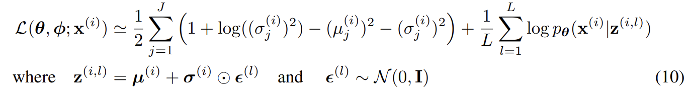
prior over the latent variables가 centered isotropic multivariate Gaussian $p_θ(z) = N (z; 0, I)$라고 두자. 이 경우 prior는 parameter가 부족하다. 우리는 $p_θ(x|z)$가 multivariate
Gaussian (in case of real-valued data)이나 Bernoulli (in case of binary data)이도록 두어 이들의 distribution parameters가 MLP (fully-connected neural network with a single hidden layer)를 가지고 z에서부터 계산될 수 있게 두었다. 이 경우 true posterior $p_θ(z|x)$는 intractable하다. form $q_φ(z|x)$에 제법 freedom이 있지만 우리는 true (but intractable) posterior가 approximately diagonal covariance를 가진 approximate Gaussian form를 맡는다고(takes on) 가정한다. 이 경우 우리는 variational approximate posterior가 diagonal covariance structure를 가진 multivariate Gaussian이도록 둘 수 있다.

approximate posterior의 mean과 s.d.는 encoding MLP의 output, 즉 datapoint $x^{(i)}와 variational parameters φ에 대한 nonlinear functions의 output이다.

앞서 설명했듯 $z^{(i,l)} = g_φ(x^{(i)}, \epsilon^{(l)}) = µ^{(i)} + σ^{(i)} \odot \epsilon^{(l)}, \epsilon^{(l)} ∼ N(0, I)$를 사용해 posterior $z^{(i,l)} ∼ q_φ(z|x^{(i)})$에서 sample한다. 이 모델에서 $p_θ(z)$ (prior)와 $q_φ(z|x)$가 모두 Gaussian이다. 이 경우 식 (7)의 estimator을 사용할 수 있고, 여기서 KL divergence는 estimation 없이 계산되고 미분될 수 있다(appendix B). 결과적으로 이 model과 datapoint $x^{(i)}$에 대한 estimator은 다음과 같다. 앞서 설명했듯 decoding term $\log p_θ(x^{(i)}|z^{(i,l)})$은 우리가 modeling하는 데이터의 종류에 따라 Bernoulli나 Gaussian MLP다.

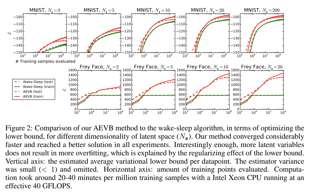
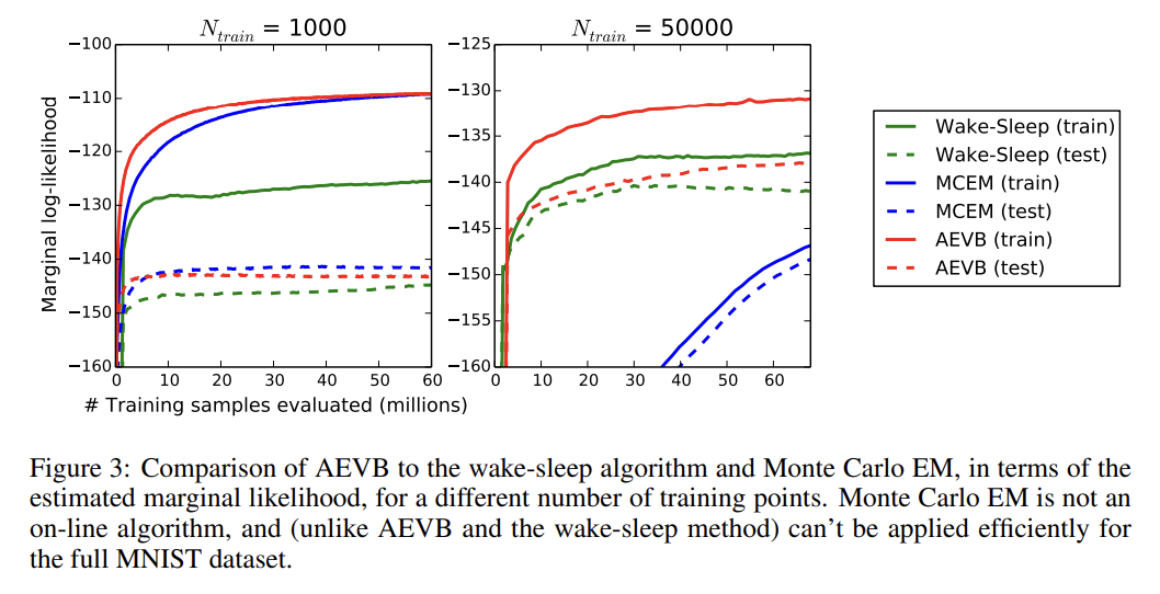
실험은 MNIST와 Frey Face datasets에 generative models를 학습시킨다. 앞서 설명한 generative model (encoder)와 variational approximation (decoder)가 사용되며 둘은 동일한 수의 hidden units를 가진다. 설명은 생략한다.

---

다른 포스트로부터 긴빠이정리한 것이다.