AN IMAGE IS WORTH 16X16 WORDS: TRANSFORMERS FOR IMAGE RECOGNITION AT SCALE

오늘 리뷰할 논문은 ViT 논문이다.

아래 포스트를 먼저 보면 도움이 될 것이다.

• [논문리뷰]AN IMAGE IS WORTH 16X16 WORDS: TRANSFORMERS FOR IMAGE RECOGNITION AT SCALE : Vi-T(Vision Transformer)
• [논문 리뷰] An Image is Worth 16x16 Words: Transformers for Image Recognition at Scale (2021)
• 쉽게 이해하는 ViT(Vision Transformer) 논문 리뷰 | An Image is Worth 16x16 Words: Transformers for Image Recognition at Scale

---

Summary

컴퓨터 비전에서 attention은 CNN와 함께 사용되거나 CNN의 전반적인 구조는 유지하면서 일부를 대체하는 식으로 사용된다. 논문은 CNN에 대한 이런 의존이 필수적이지 않으며 sequences of image patches에 직접 적용된 순수한 transformer가 image classification tasks를 잘 수행할 수 있음을 보인다. 대량의 데이터에 pre-train되고 여러 mid-sized/small image recognition benchmarks (ImageNet, CIFAR-100, VTAB, 등)로 transfer되면 Vision Transformer (ViT)은 SOTA CNN에 비해 적은 연산량만 소모하면서 훌륭한 성능을 보인다.

NLP에서 Transformer scaling의 성공에 영감을 받아 논문은 최소한의 수정을 가한 standard Transformer을 이미지에 직접 적용하는 것을 실험한다. 그러기 위해 image를 patches로 분할해 patches의 linear embeddings의 sequence를 Transformer에 input으로 넣는다. image patches는 NLP application의 tokens (words)와 같은 방식으로 다루어진다. 모델은 image classification에 지도학습으로 훈련시킨다.

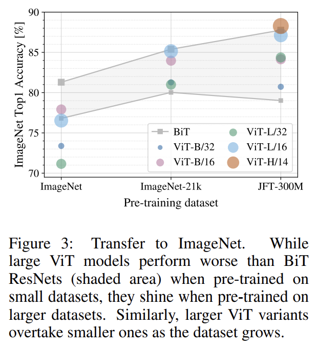
ImageNet 같은 mid-sized datasets에 강한 regularization 없이 학습된다면 ViT는 비슷한 크기의 ResNet보다 약간의(a few) percentage points 낮은 적당한(modest) 정확도를 보여준다. 겉보기엔 실망스러운 결과인데, Transformer은 CNN에 내재한 (translation equivariance와 locality 같은) 몇 inductive biases가 없기 때문에 불충분한 양의 데이터로 학습하면 일반화를 잘 못하기 때문이다.

그러나 더 큰 데이터셋에(14M-300M images) 학습되면 상황이 반전한다. 논문은 large scale training이 inductive bias를 이김(trump)을 발견했다. ViT는 충분한 scale에 pre-train되고 transfer하면 훌륭한 결과를 낸다. public ImageNet-21k dataset이나 in-house JFT-300M dataset에 학습된다면 ViT는 multiple image recognition benchmarks에서 SOTA를 이긴다.

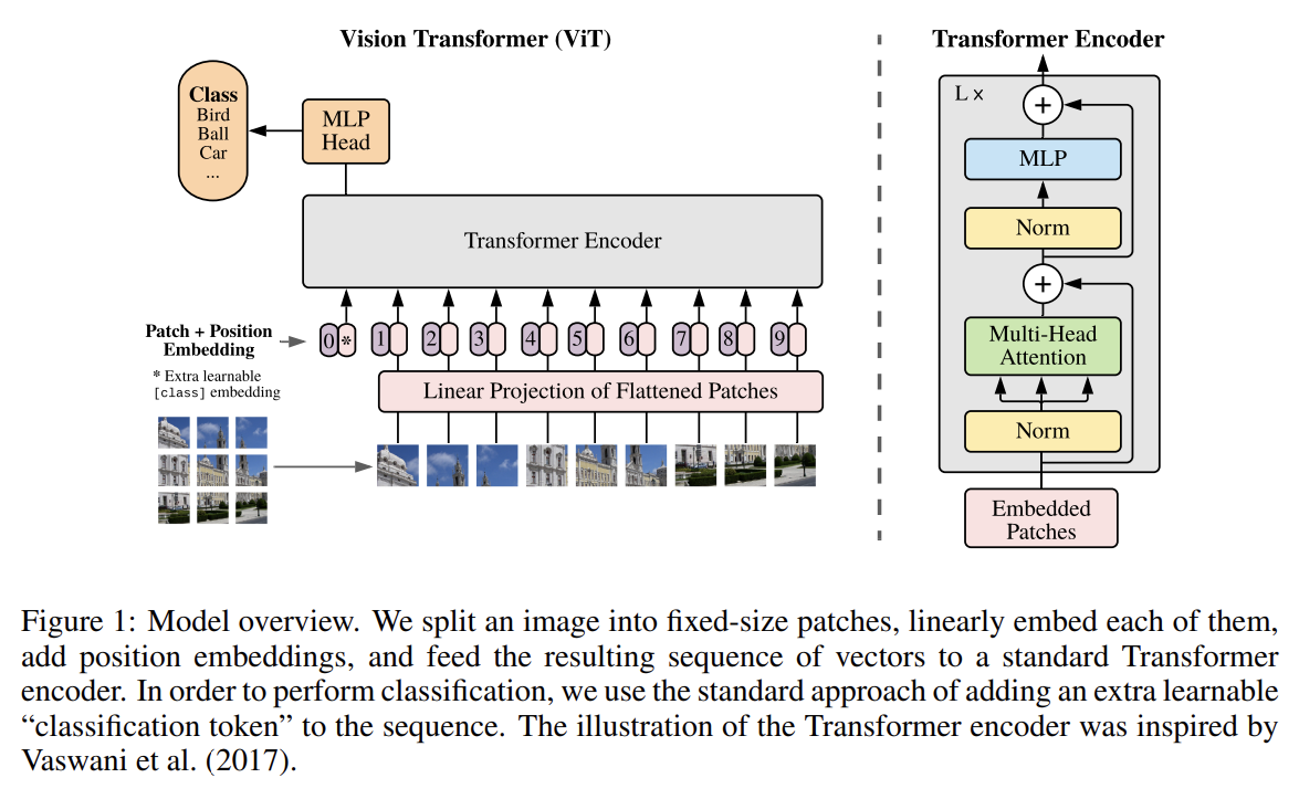
standard Transformer은 1D sequence of token embeddings을 input으로 받는다. 2D images를 다루기 위해선 image $x ∈ R^{ H×W×C}$를 sequence of flattened 2D patches $x_p ∈ R^{N×(P^2·C)}$로 reshape한다. (H, W)은 original image의 해상도, C는 channels의 수, (P, P)는 각 image patch의 해상도, $N = HW/P^2$은 (Transformer로의 effective input sequence length이기도 한) 결과적인 patches의 수다. Transformer은 모든 layer에서 constant latent vector size D을 사용하므로 trainable linear projection을(식 1) 가지고 patches을 D dimensions으로 flatten한다. 이 projection의 output을 patch embeddings이라고 부른다.

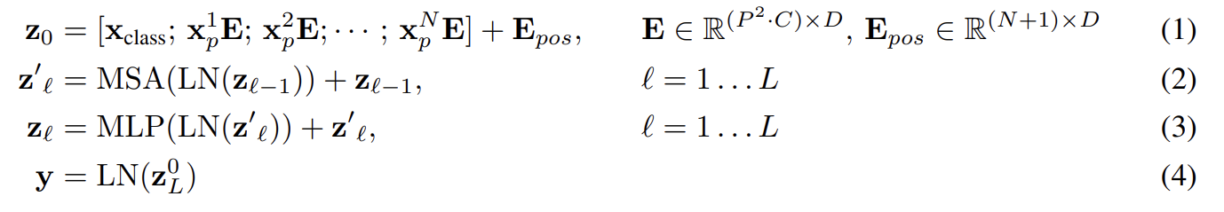
BERT의 [class] token과 비슷하게 우리는 learnable embedding을 sequence of embedded patches $(z^0_0 = x_{class})$ 앞에 붙이고(prepend), Transformer encoder의 output $z^0_L$에서 이것의 state는 image representation y로 동작한다(식 4). pre-training과 fine-tuning 둘 모두에서 classification head가 $z^0_L$에 부착된다. classification head는 pre-training time에는 one hidden layer을 가진 MLP로 구현되고 fine-tuning time에는 single linear layer로 구현된다.

positional information을 보유하기 위해 Position embeddings이 patch embeddings에 더해진다. standard learnable 1D position embeddings을 사용하는데, 발전된 2D-aware position embeddings을 사용해도 성능 향상이 크게 없었기 때문이다. 결과물인 embedding vectors의 sequence가 encoder로의 input이 된다.

Transformer encoder는 multiheaded self-attention (MSA)과 MLP blocks을 번갈아가면서 layer로 가진다(식 2, 3). 모든 block 직전에 Layernorm (LN)이 적용되고 모든 block 직후에 residual connections이 적용된다. MLP는 GELU non-linearity와 함께 2 layers로 이루어진다.

• Inductive bias

ViT가 CNN보다 훨씬 적은 image-specific inductive bias을 가짐을 유의하라. CNN에는 모델 전체에 걸쳐 locality, two-dimensional neighborhood structure, translation equivariance이 각 layer에 반영되어 있다. ViT에는 MLP layers만 local하고 translationally equivariant하며 self-attention layers은 global하다. two-dimensional neighborhood
structure은 아주 조금만 사용되었다. 모델 시작 부분에 image를 patches로 자를 때와 fine-tuning 시기에 다양한 해상도의 이미지를 위해 position embeddings을 조정할 때 사용되었다. 그걸 제외하면 initialization time에 position embeddings은 patches의 2D position에 대한 어떤 정보도 지니지 않으며 patches 사이 모든 spatial relations은 맨땅에서부터 학습되어야 한다.

• Hybrid Architecture

raw image patches에 대한 대안책으로써 input sequence이 CNN의 feature maps로부터 형성될 수 있다. 이 hybrid model에선 patch embedding projection E (식 1)이 CNN feature maps에서 추출한 patches에 적용된다. 특수한 경우로 patches는 spatial size 1x1를 가질 수 있으며 이는 input sequence가 단순히 feature map의 spatial dimension을 flatten하고 Transformer dimension로 project함으로써 구해진다는 것을 의미한다.

• FINE-TUNING AND HIGHER RESOLUTION

ViT는 큰 데이터셋에 pre-train하고 비교적 작은 downstream task에 fine-tune한다. 이를 위해 pre-trained prediction head을 제거하고 zero-initialized D × K feedforward layer을 부착한다. K는 downstream classes의 수다. 보통 pre-training보다 higher resolution에서 fine-tuning하는 편이 이롭다. higher resolution의 image를 먹일 때 patch size는 동일하게 유지하며 이는 larger effective sequence length을 초래한다. ViT는 (메모리가 허락하는 한) 임의의 sequence length도 다룰 수 있으나 그러면 pre-trained position embeddings가 더는 의미가 없어질 수도 있다. 따라서 original image 내에서 그들의(=patches) location을 기반으로 pre-trained position embeddings의 2D interpolation을 수행한다. 이 resolution adjustment과 patch extraction가 image의 2D structure에 대한 inductive bias가 수동으로 ViT에 주입되는 유일한 부분임에 주의하라.

실험은 ResNet, ViT, hybrid model의 representation learning 능력을 평가한다. 각 모델의 데이터 요구를 이해하기 위해 다양한 크기의 데이터셋에 pre-train하고 많은 benchmark tasks를 평가한다. ViT는 대부분의 recognition test에서 적은 pre-training 연산량을 가지고 SOTA를 달성한다.

(데이터셋 설명 생략)

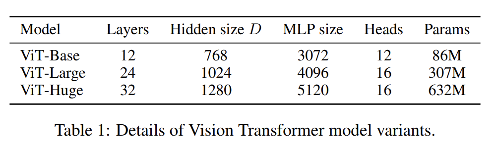
ViT 환경 설정은 BERT 논문을 기반으로 한다. Transformer의 sequence length는 patch size 제곱에 반비례하므로 더 작은 patch size를 가진 모델이 더 연산이 비싸다는 사실에 주의하라.

baseline CNN으로는 ResNet을 썼는데 Batch Normalization layer을 Group normalization으로 교체하고 standardized convolutions을 사용했다. 이 수정은 transfer을 향상시키며 모델을 “ResNet (BiT)”라고 이름붙였다. hybrid model의 경우 ViT에 one "pixel" 크기의 patch로 intermediate feature maps을 먹인다. 다양한 sequence length를 실험하기 위해 1. regular ResNet50의 stage 4의 output을 쓰거나 2. stage 4를 제거하고 stage 3에 같은 수의 layers를 위치시켜 이 extended stage 3의 output을 썼다. 2번 옵션이 4배 긴 sequence length와 더 연산적으로 비싼 ViT 모델을 초래한다.

(중략)

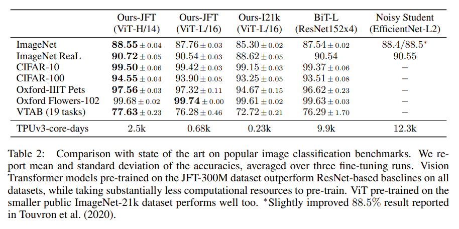
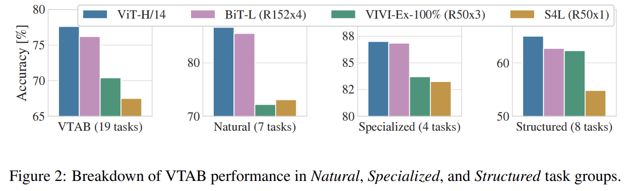
먼저 가장 큰 모델인 ViT-H/14와 ViT-L/16을 SOTA CNN 모델과 비교한다. smaller ViT-L/16 model이 동일한 데이터셋으로 pre-train된 BiT-L보다 더 적은 연산량으로 모든 task에서 더 뛰어났다. 더 큰 모델인 ViT-H/14는 성능을 더 향상시키며 여전히 기존 SOTA보다 연산량이 적었다. 그러나 pre-training efficiency은 model architecture뿐 아니라 training schedule, optimizer, weight decay 등 다른 변수에도 영향을 받음을 주의하라.

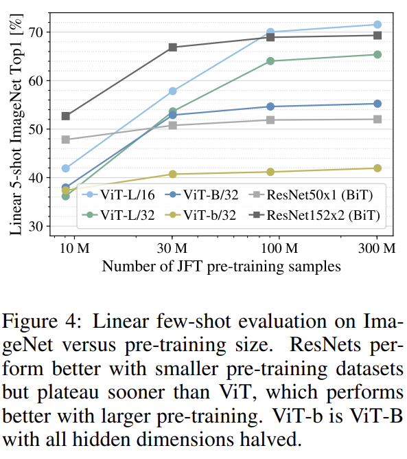
데이터셋 크기의 영향도 실험했다.

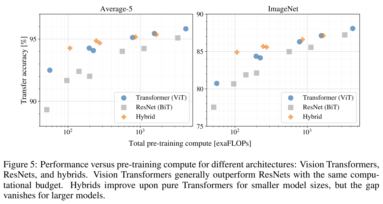
scaling study로 transfer performance versus total pre-training cost도 실험한다. 몇 가지 패턴이 관측된다. 첫째로 performance/compute trade-off에서 ViT가 ResNet을 압도했다. ViT는 (5 데이터셋 평균을 기준으로) 동일한 성능을 내기 위해 2-4배 적은 연산량을 사용했다. 둘째로 small computational budgets에서 hybrids가 ViT보다 약간 성능이 좋았으나 larger model에선 차이가 사라졌다. 이 결과는 흥미로운데, convolutional local feature processing가 모든 size에서 ViT를 돕든다고 예상할 수 있기 때문이다. 셋째로 시도한 범위 내에서 ViT는 포화하지 않았고 향후 scaling 연구에 동기를 부여한다.

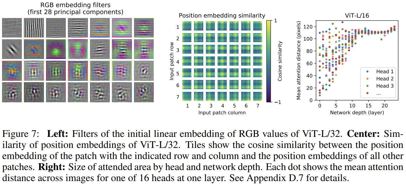
ViT가 어떻게 이미지 데이터를 처리하는지 이해하기 위해 internal representations을 분석했다. ViT의 첫 layer은 flattened patches를 lower-dimensional space로 linearly project한다(식 1). Fig 7 왼쪽은 learned embedding filters의 top principal components를 보여준다. components들은 (각 patch 내의 fine structure의) low-dimensional representation에 대한 plausible basis functions을 닮았다.

projection 이후 patch representations에 learned position embedding가 더해진다. Fig 7 중앙은 모델이 position embeddings similarity에서 image 내의 distance를 encode하도록 학습됨을 보여준다. 즉, closer patches는 더 비슷한 position embeddings을 가진다는 것이다. 또 row-column structure가 나타나는데 같은 row/columns에 위치한 patches는 비슷한 embeddings을 가진다. 마지막으로 larger grids에는 가끔 sinusoidal structure 이 나타난다. position embeddings이 2D image topology를 표현하도록 학습한다는 사실은 왜 position embeddings이 성능 향상을 만들지 않는지 보여준다.

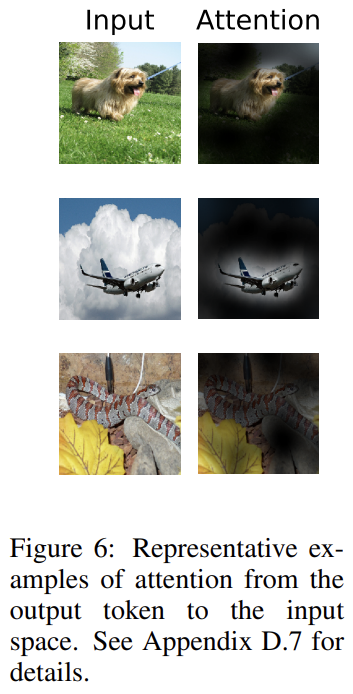
Self-attention은 (심지어 lowest layer에서도) ViT가 이미지 전체에 걸쳐 정보를 통합하게 해준다. 네트워크가 이 능력을 어느 정도나 사용하는지 실험한다. 구체적으로는 attention weights에 기반해 image space 내에서 정보가 통합되는 average distance을 측정한다. 이 “attention distance”은 CNN의 receptive field size와 유사하다(analogous). Fi 7 오른쪽에서 몇 heads가 이미 lowest layers에서 이미지 대부분에 attend하는 것을 발견해 정보를 통합하는 능력이 모델에 사용됨을 확인했다. 다른 attention heads는 low layer에서 일관적으로 작은 attention distances를 가진다. 이 highly localized attention은 Transformer 이전에 ResNet을 적용하는 hybrid model에서 덜 나타났다. 이는 highly localized attention이 CNN의 early convolutional layers와 비슷한 기능을 함을 주장한다. 또 network depth에 따라 attention distance이 증가했다. Fig 6에서 모델이 classification을 위해 의미적으로 연관된 이미지 영역을 attend함을 발견했다.

Strengths

1. CV에 self-attention을 사용하는 기존 연구와 달리 initial patch extraction step을 제외하면 image-specific inductive biases을 도입하지 않았다.
2. Transformer 기반이라 연산이 효율적이고 확장성(scalability)이 좋다. input sequence의 길이에 구애받지 않는다.

Weaknesses

1. 결론 부분의 뉘앙스를 보니 detection과 segmentation 같은 다른 CV task에는 성능이 썩 좋지 않은 듯하다.

---

inductive bias라는 용어가 뭔지 몰랐는데 여기에 잘 설명되어 있다.