앙상블 기법

• Voting, Bagging, Boosting, 스태깅
• Voting 은 전체데이터셋 하나로 각기 다른 모델 사용
• Bagging 계열의 앙상블 기법은 Decision Tree 사용. 하나의 데이터셋 나누어서 사용. 데이터 중복 허용
  

로지스틱 회귀

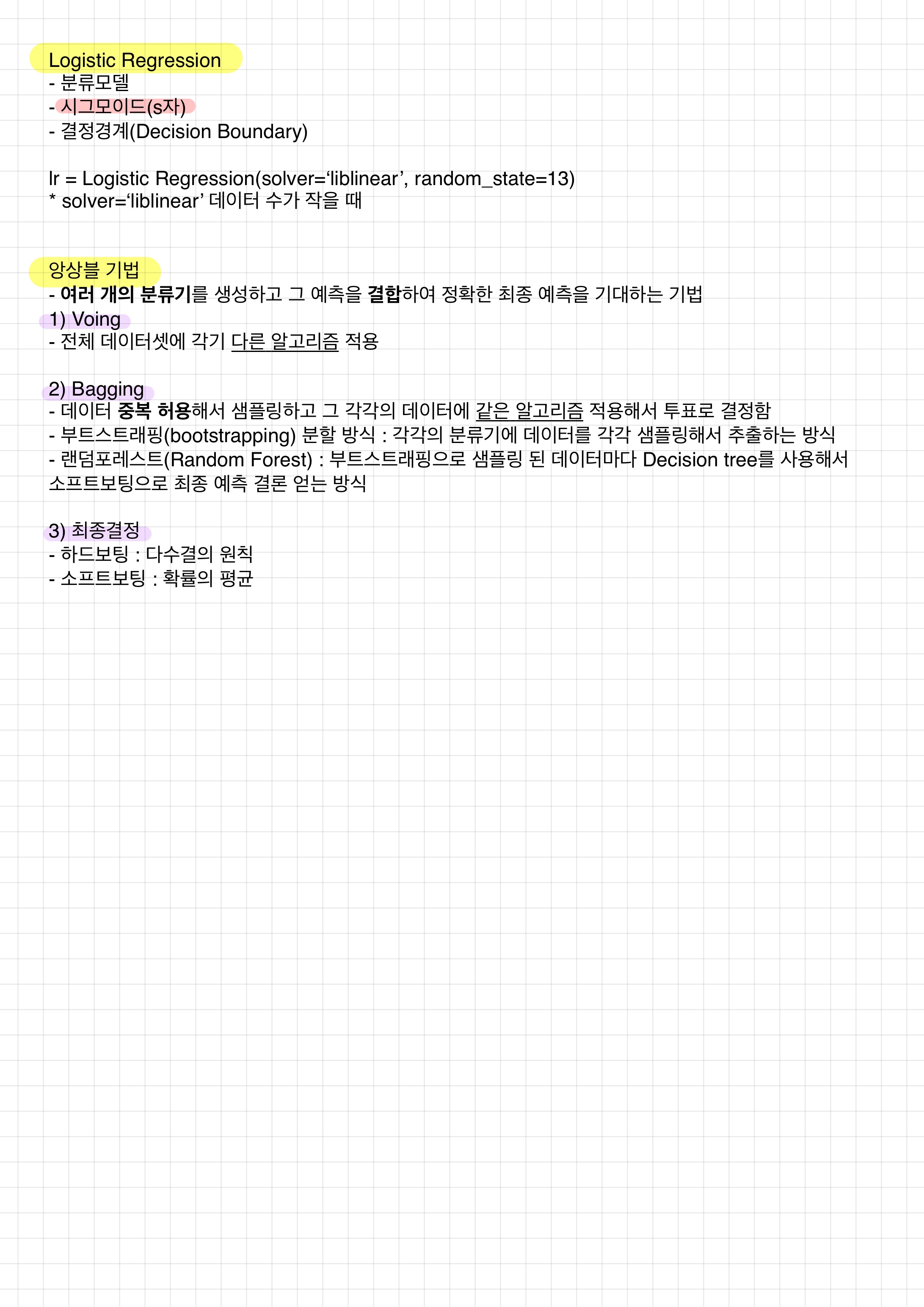
시그모이드 함수 그리기

import pandas as pd
import numpy as np
import matplotlib.pyplot as plt
%matplotlib inline

z = np.arange(-10, 10, 0.01)
g = 1 / ( 1+np.exp(-z))

plt.figure(figsize=(8,5))
ax = plt.gca()

ax.plot(z, g)
ax.spines['left'].set_position('zero')
ax.spines['right'].set_color('none')
ax.spines['bottom'].set_position('center')
ax.spines['top'].set_color('none')

plt.show()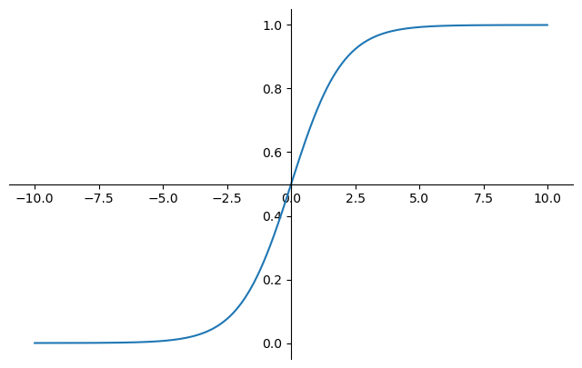

로지스틱 회귀 Cost function

h = np.arange(0.01, 1, 0.01)

C0 = -np.log(1-h)
C1 = -np.log(h)

plt.figure(figsize=(8,5))
plt.plot(h, C0, label='y=0')
plt.plot(h, C1, label='y=1')
plt.legend(loc='upper right')

plt.show()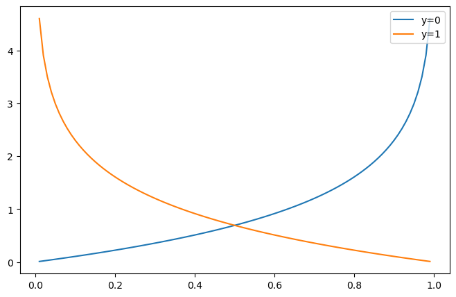

와인 데이터 분석

LogisticRegression

from sklearn.model_selection import train_test_split
from sklearn.linear_model import LogisticRegression
from sklearn.metrics import accuracy_score

X = wine.drop(['taste', 'quality'], axis=1)
y = wine['taste']

X_train, X_test, y_train, y_test = train_test_split(X, y, test_size=0.2, random_state=13)

lr = LogisticRegression(solver='liblinear', random_state=13)
lr.fit(X_train, y_train)

y_pred_tr = lr.predict(X_train)
y_pred_test = lr.predict(X_test)

print(accuracy_score(y_train, y_pred_tr))  # 0.7429286126611506
print(accuracy_score(y_test, y_pred_test)) # 0.7446153846153846

classification_report

from sklearn.metrics import classification_report
print(classification_report(y_test, y_pred_test))

confusion_matrix

from sklearn.metrics import confusion_matrix
confusion_matrix(y_test, y_pred_test)

# array([[275, 202],
#       [130, 693]])

precision_recall_curve

from sklearn.metrics import precision_recall_curve

plt.figure(figsize=(8,5))
pred = lr.predict_proba(X_test)[:,1]
precisions, recalls, thresholds = precision_recall_curve(y_test, pred)

plt.plot(thresholds, precisions[:len(thresholds)], label="precision")
plt.plot(thresholds, recalls[:len(thresholds)], label="recall")

plt.grid()
plt.legend()
plt.show()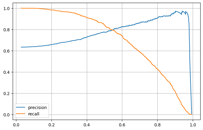

정밀도와 재현율(Precision, Recall) 트레이드오프

from sklearn.preprocessing import Binarizer

pred_proba = lr.predict_proba(X_test)

# pred_proba, y_pred_test 합치기
np.concatenate([pred_proba, y_pred_test.reshape(-1,1)], axis=1)

# threshold 바꿔 보기(Binarizer)
binarizer = Binarizer(threshold=0.6).fit(pred_proba)
pred_bin = binarizer.transform(pred_proba)[:,1]

# 다시 classification
print(classification_report(y_test, pred_bin))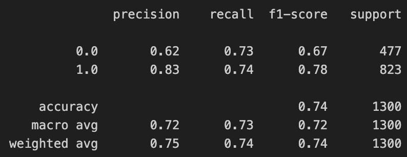

Pipeline

from sklearn.pipeline import Pipeline
from sklearn.preprocessing import StandardScaler

estimators = [('scaler', StandardScaler()),
              ('clf', LogisticRegression(solver='liblinear', random_state=13))]

pipe = Pipeline(estimators)

pipe.fit(X_train, y_train)

y_pred_tr = pipe.predict(X_train)
y_pred_test = pipe.predict(X_test)

print(accuracy_score(y_train, y_pred_tr)) # 0.7444679622859341 
print(accuracy_score(y_test, y_pred_test)) # 0.7469230769230769

Decision Tree와 비교

from sklearn.tree import DecisionTreeClassifier
from sklearn.metrics import roc_curve

wine_tree = DecisionTreeClassifier(max_depth=2, random_state=13)
wine_tree.fit(X_train, y_train)

models = {'logistic regression':pipe, 'decission tree':wine_tree}

# AUC 그래프
plt.figure(figsize=(8,5))
plt.plot([0,1],[0,1], label='random_guess')

for model_name, model in models.items():
    pred = model.predict_proba(X_test)[:, 1]
    fpr, tpr, thresholds = roc_curve(y_test, pred)
    plt.plot(fpr, tpr, label=model_name)

plt.grid()
plt.legend()
plt.show()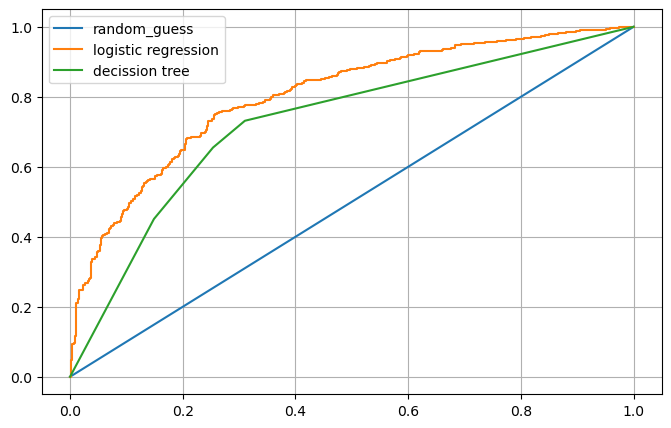

PIMA 인디언 당뇨병 예측

pima_url = 'https://raw.githubusercontent.com/PinkWink/ML_tutorial/master/dataset/diabetes.csv'
pima = pd.read_csv(pima_url)
pima = pima.astype('float')

상관관계

import seaborn as sns

sns.heatmap(pima.corr(), cmap='YlGnBu')
plt.show()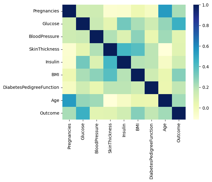

로지스틱 분석(pipeline)

# 확인
(pima==0).astype(int).sum()

# 평균값으로 대체
zero_features = ['Glucose','BloodPressure','SkinThickness','BMI']
pima[zero_features] = pima[zero_features].replace(0, pima[zero_features].mean())

X = pima.drop(['Outcome'], axis=1)
y = pima['Outcome']

X_train, X_test, y_train, y_test = train_test_split(X, y, test_size=0.2, random_state=13, stratify=y)

# pipeline
estimators = [('scaler', StandardScaler()),
              ('clf', LogisticRegression(solver='liblinear', random_state=13))]

pipe_lr = Pipeline(estimators)
pipe_lr.fit(X_train, y_train)
pred = pipe_lr.predict(X_test)

from sklearn.metrics import (accuracy_score, recall_score, precision_score, roc_auc_score, f1_score)

print('accuracy : ', accuracy_score(y_test, pred))
print('recall : ', recall_score(y_test, pred))
print('precision : ', precision_score(y_test, pred))
print('auc : ', roc_auc_score(y_test, pred))
print('f1 : ', f1_score(y_test, pred))

# accuracy :  0.7727272727272727
# recall :  0.6111111111111112
# precision :  0.7021276595744681
# auc :  0.7355555555555556
# f1 :  0.6534653465346535

상관계수(coef)

# 중요도 확인(coef)
coef = list(pipe_lr['clf'].coef_[0])
labels=list(X_train.columns)

# 중요도 데이터프레임 만들기
features = pd.DataFrame({'Features':labels, 'importance':coef})
features.sort_values(by='importance', ascending=True, inplace=True)
features['positive'] = features['importance']>0
features.set_index('Features', inplace=True)

# 시각화
features['importance'].plot(kind='barh', 
                            figsize=(8,5),
                            color=features['positive'].map({True:'blue', False:'red'}))
plt.xlabel('Importance')
plt.show()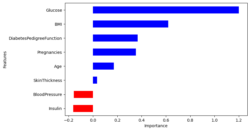

앙상블 기법(HAR 데이터)

url = 'https://raw.githubusercontent.com/PinkWink/ML_tutorial/master/dataset/HAR_dataset/features.txt'
feature_name_df = pd.read_csv(url, sep='\s+', header=None, names=['column_index','column_name'])

# feature_name
feature_name = feature_name_df.iloc[:,1].values.tolist()

X_train_url = 'https://raw.githubusercontent.com/PinkWink/ML_tutorial/master/dataset/HAR_dataset/train/X_train.txt'
X_test_url = 'https://raw.githubusercontent.com/PinkWink/ML_tutorial/master/dataset/HAR_dataset/test/X_test.txt'

X_train = pd.read_csv(X_train_url, sep='\s+', header=None)
X_test = pd.read_csv(X_test_url, sep='\s+', header=None)

X_train.columns = feature_name
X_test.columns = feature_name

y_train_url = 'https://raw.githubusercontent.com/PinkWink/ML_tutorial/master/dataset/HAR_dataset/train/y_train.txt'
y_test_url = 'https://raw.githubusercontent.com/PinkWink/ML_tutorial/master/dataset/HAR_dataset/test/y_test.txt'

y_train = pd.read_csv(y_train_url, sep='\s+', header=None, names=['action'])
y_test = pd.read_csv(y_test_url, sep='\s+', header=None, names=['action'])

y_train['action'].value_counts()
# 6    1407
# 5    1374
# 4    1286
# 1    1226
# 2    1073
# 3     986

DecisionTreeClassifier

from sklearn.tree import DecisionTreeClassifier
from sklearn.metrics import accuracy_score

dt_clf = DecisionTreeClassifier(max_depth=4, random_state=13)
dt_clf.fit(X_train, y_train)
pred = dt_clf.predict(X_test)
accuracy_score(y_test, pred)   # 0.8096369189005769

# GridSearchCV
from sklearn.model_selection import GridSearchCV

params = {'max_depth' : [6,8,10,12,16,20,24]}

grid_cv = GridSearchCV(dt_clf, param_grid=params, scoring='accuracy', cv=5, return_train_score=True)
grid_cv.fit(X_train, y_train)

grid_cv.best_score_    # 0.8543335321892183
grid_cv.best_params_   # {'max_depth': 8}

cv_results_df = pd.DataFrame(grid_cv.cv_results_)
cv_results_df[['param_max_depth','mean_test_score','mean_train_score']]

# 가장 예측력 좋은 모델에 테스트
best_dt_clf = grid_cv.best_estimator_
pred1 = best_dt_clf.predict(X_test)

accuracy_score(y_test, pred1)   # 0.8734306073973532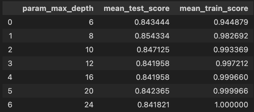

RandomForestClassifier

from sklearn.ensemble import RandomForestClassifier

params = {
    'max_depth':[6,8,10],
    'n_estimators':[50,100,200],  # Decision Tree를 몇 그루 사용할지
    'min_samples_leaf':[8,12],  # 최소 데이터모음 수
    'min_samples_split':[8,12]
}

rf_clf = RandomForestClassifier(random_state=13, n_jobs=-1)
grid_cv = GridSearchCV(rf_clf, param_grid=params, cv=2, n_jobs=-1)
grid_cv.fit(X_train, y_train)

cv_results_df = pd.DataFrame(grid_cv.cv_results_)
target_cols = ['rank_test_score','mean_test_score','param_n_estimators','param_max_depth']
cv_results_df[target_cols].sort_values(by='rank_test_score').head()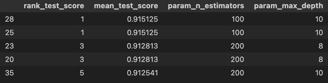

print(grid_cv.best_estimator_)
# RandomForestClassifier(max_depth=10, min_samples_leaf=8, min_samples_split=8,
#                        n_jobs=-1, random_state=13)

print(grid_cv.best_score_)  # 0.9151251360174102

# 가장 예측력 좋은 모델에 학습&테스트 
rf_clf_best = grid_cv.best_estimator_
rf_clf_best.fit(X_train, y_train)

pred = rf_clf_best.predict(X_test)
accuracy_score(y_test, pred)  # 0.9205972175093315

중요 특성 추출(featureimportances)

best_cols_values = rf_clf_best.feature_importances_
best_cols = pd.Series(best_cols_values, index=X_train.columns)
top20_cols = best_cols.sort_values(ascending=False)[:20]

# 시각화
plt.figure(figsize=(8,8))
sns.barplot(x=top20_cols, y=top20_cols.index)
plt.show()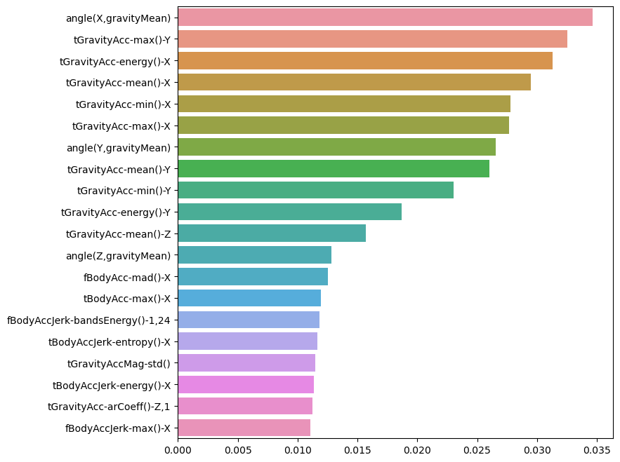

# 20개 특성만 가지고 다시 성능 확인
X_train_re = X_train[top20_cols.index]
X_test_re = X_test[top20_cols.index]

rf_clf_best_re = grid_cv.best_estimator_
rf_clf_best_re.fit(X_train_re, y_train.values.reshape(-1,))

pred1_re = rf_clf_best_re.predict(X_test_re)

accuracy_score(y_test, pred1_re)  # 0.8177807940278249