[ArXiv2018]Learning Confidence for Out-of-Distribution Detection in Neural Networks - [2022.08.01]

논문의 저자는 다음과 같이 설명한다.

To jointly address these issues, we propose a method of learning confidence estimates for neural networks that is simple to implement and produces intuitively interpretable outputs.

Additionally, we address the problem of calibrating out-of-distribution detectors. where we demonstrate that misclassified in-distribution examples can be used as a proxy for out-of-distribution examples.

위 두 내용이 핵심 내용이다.

먼저 네트워크가 confidence estimates라는 것을 학습시킬 수 있도록 네트워크를 구성한다. 덧붙여서 misclassified in-distribution examples를 통해 out-of-distribution examples의 역할을 만드는 것이 목표이다.

---

What do you get if you multiply six by nine? How many roads must a man walk down? What is the meaning of life, the universe, and everything?

이러한 질문들은 누군가에게는 굉장히 자신감 있게 대답할 수도 있지만 어떤 이들에게는 어느정도 불확실한 대답을 할 수 있을 것이다. 우리 스스로 이해하고 있는 것에 대한 한계(Knowing the limitations of one's own understanding)에 대해 아는 아는 것은 의사 결정에 매우 중요하다. 이러한 정보는 측정하기 원하고 잠재적인 위험을 줄일 수 있다.

이게 바로 Uncertainty이다. 이 논문에서는 Uncertainty문제를 Confidence관점에서 설명하고 있고, 네트워크 자체에서 이를 출력하도록 만든다. 그리고 이러한 confidence를 통해서 out-of-distribution문제를 해결하고자 한다.

---

Confidence Estiation

Confidence Estimation과 out-of-distribution은 비슷한 부분들이 존재한다. 우리가 모델을 학습시킬 때, 새로운 데이터가 네트워크의 입력으로 들어왔을 때 Confidence 값이 일반적으로 낮을 것을 기대한다. 이런 것처럼 well calibrated confidence estimates는 out-of-distribution을 구분하는 것이 가능해진다. 이상적으로 confidence를 각각의 입력에서 직접적으로 측정하기를 원한다. 그러나 이건 대부분의 머신러닝 문제에서 입증하기 어렵고, 이러한 confidence에 대한 ground truth label이 존재하지 않는다는 어려움이 있다.

직접적으로 confidence를 학습하는 것 대신에, 본 논문의 저자들은 새로운 방법으로 네트워크를 훈련하는 동안 confidence estimates를 생성하도록 만든다.

이 때 이 confidence estimates는 주어진 입력에 대해서 올바른 예측을 할 수 있는 능력을 반영한다.

Motivation

Imagine a test writing scenario, For this particular test, the student is given the option to ask for hints, but for each hint they receive, they also incur some small penalty. In order to optimize their score on the test, a good strategy would be to answer all of the questions that they are confident in without using the hints, and then to ask for hints to the questions that they are uncertain about in order to improve their chances of answering them correctly.

한가지 예시를 들어보자.

어떤 시험을 친다고 하였을 때, 학생은 힌트를 옵션으로 얻을 수 있다. 그러나 그 힌트를 받았을 때 약간의 페널티를 받게 된다. 테스트의 점수를 최적화 하기 위해서, 가장 좋은 전략은 힌트 없이 모든 문제를 맞추는 것이겠지만, 힌트가 없으면 틀릴수 있기 때문에 적절하게 힌트를 사용하여 문제를 해결해야 한다. 이 때, 그러면 힌트를 얻을 만한 문제에 대해 알아내기 위한 지표가 Uncertainty가 될 것이다.

---

Learning to Estimate Confidence

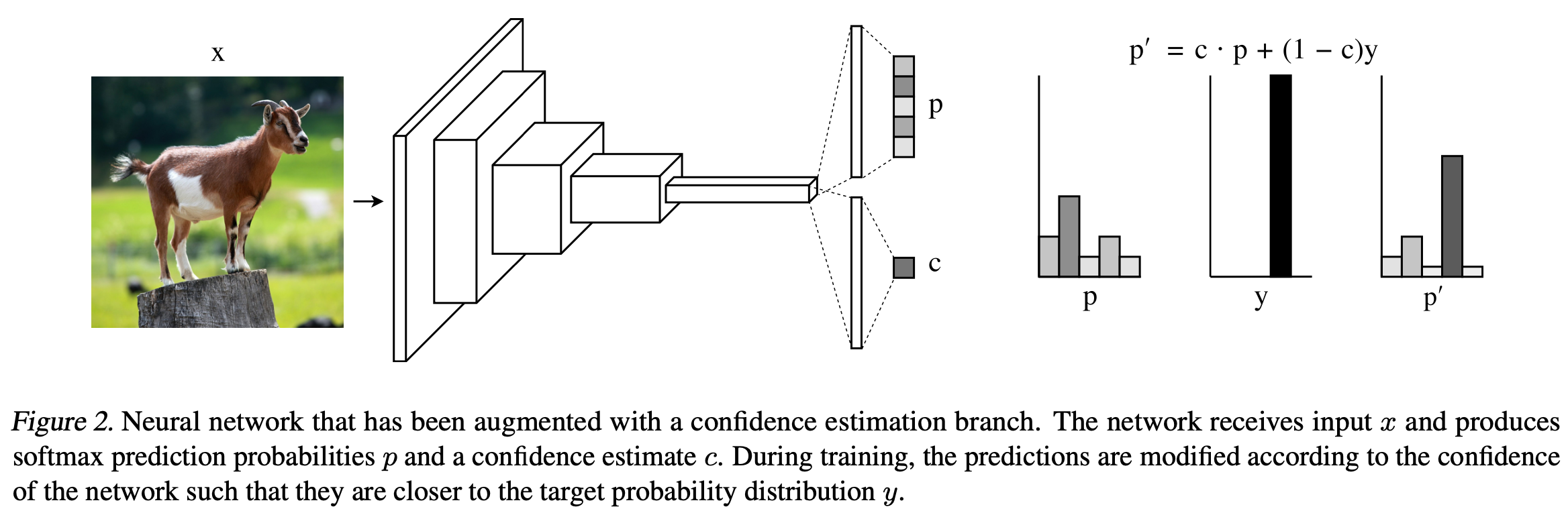
In order to give neural networks the ability to ask for hints, we first add a confidence estimation branch to any conventional feedforward architecture in parallel with the original class prediction branch, as shown in Figure 2.

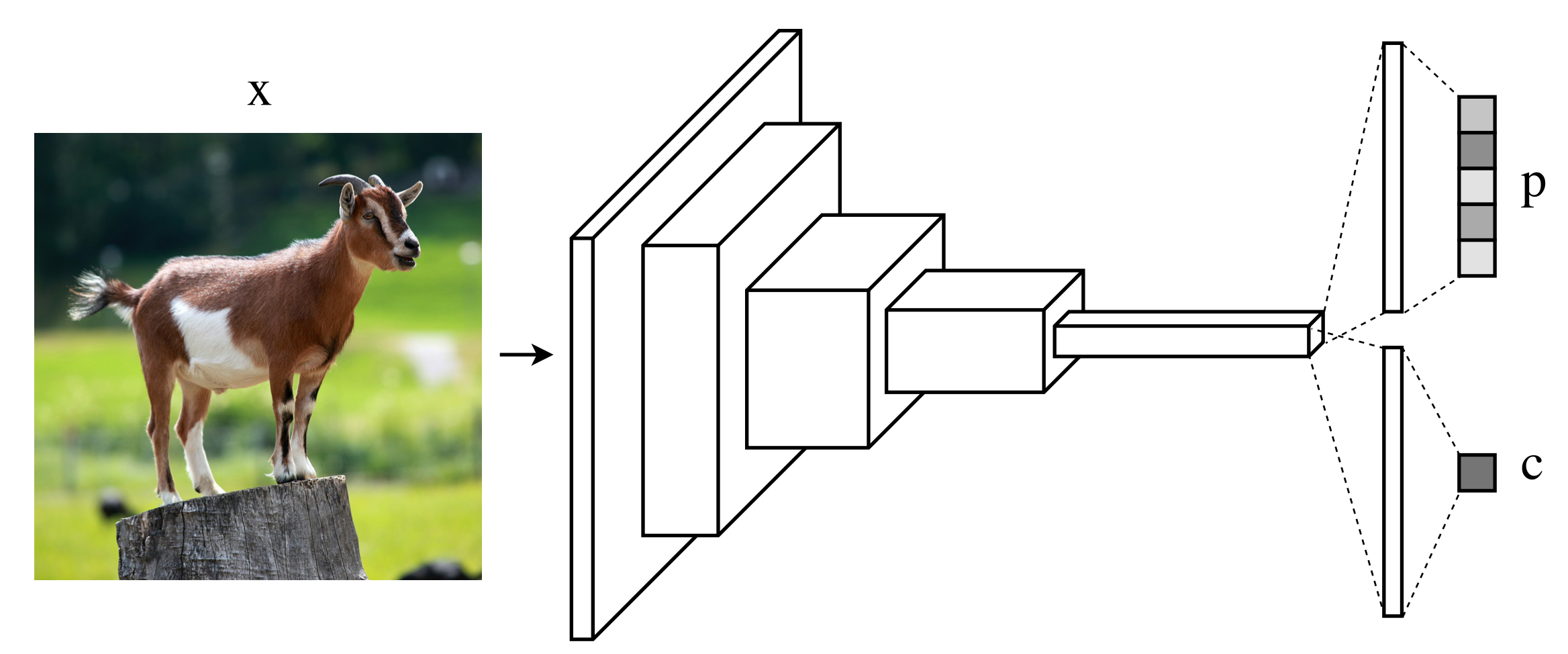
위 그림과 같이, 일반적인 neural network에 class prediction branch와 함께 confidence estimation branch를 넣어준다.

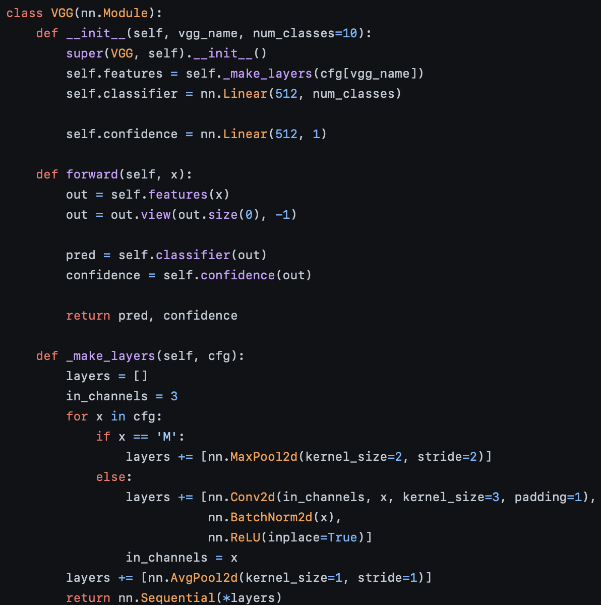
코드 상으로는 __init__에서 피처를 뽑는 _make_layers_를 두고 classifier의 Linear Layer (output == # of class)와 confidence의 Linear Layer (output == 1)를 구현하여 피처 네트워크를 통과한 피터들에 대해 confidence estimation branch와 class prediction branch를 함께 넣어준다.

In practice, the confidence estimation branch is usually added after the pernultimate layer of the original network, such that both the confidence branch and the prediction branch receive the same input.

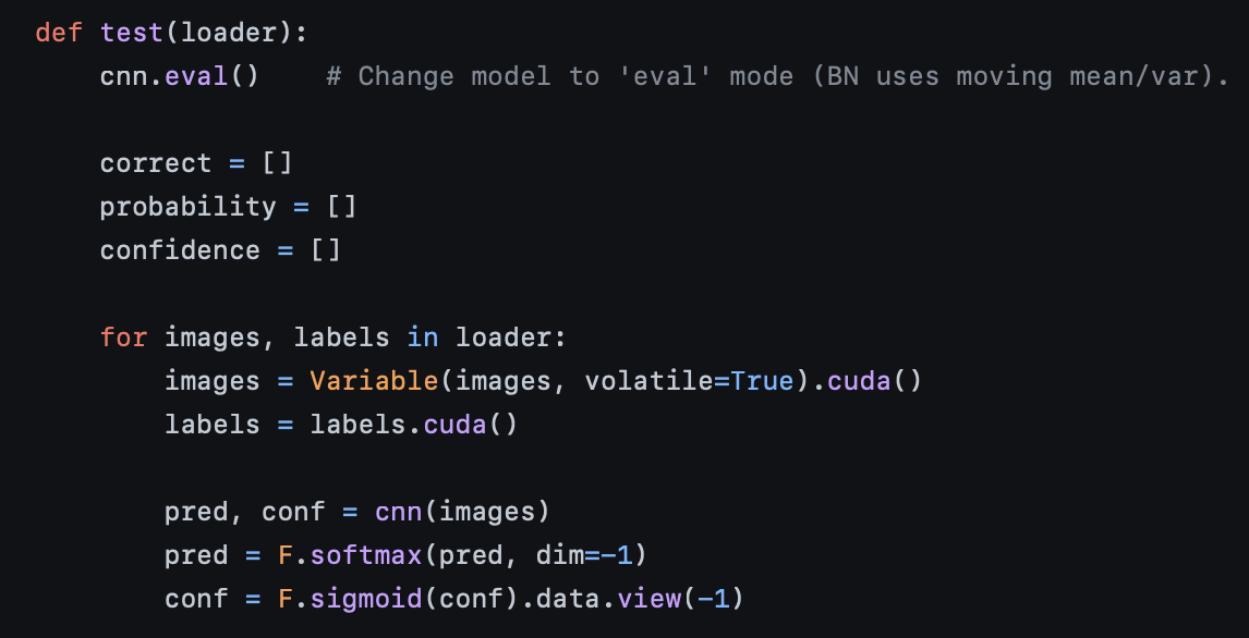
위 코드를 보면, cnn(VGG)에서 나온 결과값인 pred와 conf값을 prediction값에는 softmax함수를 취해주고, confidence 값에 대해서는 sigmoid를 취해준다. 이유는 아래와 같다.

The confidence branch contains one or more fully-connected layers, with the final layer outputting a single scalar between 0 and 1 (parametrized as a sigmoid). This confidence value c represents the network's confidence that it can correctly produce the target output given som input.

confidence라고 불리는 우리의 예측을 0과 1사이의 어떤 수로 정의하고, 이를 이용해서 모델(CNN network)가 입력에 대해 나오는 결과값에 따라 모델의 confidence를 측정하겠다는 의미가 담겨있다.

If the network is confident that it can produce a correct prediction for the given input, it should output $c$ close to 1. Conversely, if the network is not confidence that it can produce the correct prediction, then it should output $c$ close to 0.

간단하게 설명하면, 만약에 network가 입력 값에 대한 예측이 옳을 것이라고 자신(confidence)이 잇다면 $c$가 1로 수렴할 것이고, 만약 예측이 옳지 않을 것이라고 자신없다면, $c$가 0으로 수렴할 것이다.

수식으로 표현하면 아래와 같다.

$p, c = f(x,\Theta)$,$p_i,c\in{[0,1]},\Sigma^M_{i=1}p_i=1$.

In order to give the network "hints" during training, the softmax prediction probabilities are adjusted by interpolating between the original predictions and the target probability distribution $y$, where the degree of interpolation is indicated by the network's confidence:

$p'_i=c\cdot{p_i}+(1-c)y_i$.

여기가 핵심인데,

$c$는 그냥 0부터 1사이의 어떤 값으로 나올텐데, 자신이 있을 때$c$값을 높이고, 자신이 없을 때 $c$값을 낮추기 위해 위와 같은 식으로 아주 간단하게 표현했다.

내가 내놓는 예측값과 실제 타겟 값의 interpolation값을 예측 값 $p'_i$로 두고 이 예측값으로 로스를 주었다.

$\mathcal{L}_t = -\Sigma^M_{i=1}\log{(p'_i)y_i}$

그런데 위 loss만 사용했을 때 문제가 발생한다.

loss를 최소화 하기 위해서, 계속해서 힌트만을 보는 것이다. 이를 막기 위해서, $c$에 대한 로스를 주어, confidence가 최대한 높게 나오도록 학습시킨다.

$\mathcal{L}_c=-\log(c)$

이 둘을 합쳐 최종 로스를 구한다.

$\mathcal{L=L_t+\lambda{L_c}}$

We can now investigate how the confidence score impacts the dynamics of the loss function. In cases where $c\rightarrow{1}$ (i.e., the network is very confident), we see that $p'\rightarrow{p}$ and the confidence loss goes to 0.This is equivalent to training a standard network without a confidence branch. In the case where $c\rightarrow{0}$ (i.e. the network is not very confident), we see that $p'\rightarrow{y}$, so the network receives the correct label. In this scenario the task loss will go to 0, but the confidence loss becomes very large. Finally, if $c$ is some value between 0 and 1, then $p'$ will be pushed closer to the target probabilities, resulting in a reduction in the task loss at the cost of an increase in the confidence loss. This interaction produces an interesting optimization problem, wherein the network can reduce its overall loss if it can successfully predict which inputs it is likely to classify incorrectly.

상황에 대해 간단하게 설명한다.

만약에 $c\rightarrow{1}$인 경우는 $p'\rightarrow{p}$로 가기 때문에, $\mathcal{L_c=-\log{c}}$ 값은 0으로 수렴한다.

반대의 경우 $c\rightarrow{0}$인 경우는 $p'\rightarrow{y}$로 가기 때문에, $\mathcal{L}_t = -\Sigma^M_{i=1}\log{(p'_i)y_i}$ 값은 0으로 수렴한지만 confidence loss가 커진다.

이 상호 작용이 재밌는 optimization 문제를 만들어 낸다. -> 보완할 점이 있어 보인다.

---

Implementation Details

위 까지는 메소드에 대한 설명이고, 실험을 하기 위한 구체적인 설정들에 대해 알아보도록 하자.

It requires several optimizations to make it robust across datasets and architectures. These include methods for automatically selecting the best value for $\lambda$ during training, combating excessive regularization that reduces classification accuracy, and retaining miscalssified examples throughout training.

로스를 최적화하여 dataset and architectures에 robust한 모델을 만들기 위해서, 여러가지 메소드를 사용한다.

1. Budget Parameter
2. Combating Excessive Regularization
3. Retaining Misclassified Examples

---

Budget Parameter

---

Combating Excessive Regularization

---

Retaining Misclassified Examples

---