Time Series Anomaly Detection with Multiresolution Ensemble Decoding

Time Series Anomaly Detection with Multiresolution Ensemble Decoding

• 2021 AAAI Conference on Artificial Intelligence (AAAI-21)

RNN based autoencoder with decoder ensembles

기존 RNN을 사용한 autoencoder는 sequential decoding으로 인해 overfitting 및 error accumulation이 발생하기 쉬움
➜ decoding length가 다른 여러 개의 decoder를 사용하는 방법을 적용

Introduction

previous recurrent auto-encoder based anomaly detection methods
➜ privious time steps로 인한 error accumulation 때문에 long time series를 reconstruction 하는데 어려움이 존재할 수 있음

• error accumulation : decoder의 input으로 이전 시점의 output이 사용되면서 이전 시점에 존재하던 error가 축적되는 문제

본 논문에서는 reccurent based multi-resolution decoders를 사용한 Multi-Resolution Ensemble Decoding(RAMED)을 제안

RAMED는 각각 다른 time step을 가지는 decoder를 사용하여 다양한 temporal information을 얻음

• short decoding length : focus on macro temporal characteristics

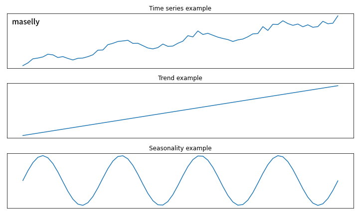
  • trend patterns
  • seasonality

• long decoding length : focus on more detailed local temporal patterns

Trend and Seasonality example

출처 : my notebook

S-RNN(S-RNN review)과 달리 lower-resolution temporal information을 higher resolution decoder에 전달

Contriution

• 서로 다른 decoding length를 가지는 multiple decoders ensemble

• 서로 다른 multiresolution temporal information을 융합하기 위한 mechanism

Architecture

Notation

Input time series : $X = [x_1, x_2, ...\:, x_{T}]$, where $x_t\in \mathbb{R}^{d}$
Output reconstructed time series : $Y = [y_T, y_{T-1}, ...\:, y_1]$ , where $y_t \in \mathbb{R}^{d}$
Error : $e(t) = y_t - x_t$
the number of encoders : $L^{(E)}$
the number of decoders : $L^{(D)}$
small noise : $\epsilon \delta$ ($\epsilon = 10^{-4}$, random noise $\delta$~$N(0,1)$)

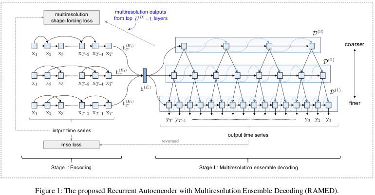
Multiresolution Ensemble Decoding

본 논문에서는 RNN을 사용한 S-RNN과 달리 LSTM을 사용

Encoding process는 S-RNN과 동일
sparsely connected RNN을 사용하는 encoder ensemble 사용
본 논문에서는 총 3개의 encoder 사용

$h^{(E)} = F_{MLP}(concat[h_{T}^{(E_1)}; ...\:;h_{T}^{(E_i)}; ...\:; h_{T}^{(E_{L(E)})} ])$
$F_{MLP}$ : fully-connected layer

Decoding process

coarser decoder의 hidden state와 finer decoder의 hidden state를 concat하여 output 도출

각 decoder가 서로 다른 temporal information을 잡아낼 수 있도록 서로 다른 수의 step을 사용

robustness를 위해 small noise를 input에 추가

decoding length	temporal characteristic
short	macro
long	micro

서로 다른 길이의 decoded output을 dynamic time warping(DTW)를 통해 input time series와 비슷하게 만듦

Decoder Lengths

$k$th decoder $D^{(k)}$ reconstructs a time series of length $T^{(k)}$, where $T^{(k)} = \alpha_{k}T$

$\alpha_{k} = \frac{1}{\tau^{k-1}} \in (0, 1]$

단,

1. $\tau > 1$

   • $\tau = 2$ in model figure

2. $\alpha_{1} = 1$ and $T^{(1)} = T$

3. $T^{(L^{(D)})} \geq 2$
   ➜ 가장 top decoder가 적어도 2 steps는 가지도록 설정

Coarse-to-Fine Fusion

outputs의 length가 각각 다르기 때문에 average or median으로 ensemble output을 정리할 수 없음
이를 위해 coarse-to-fusion strategy 사용
아래는 example

두 decoder $D^{(k+1)}$과 $D^{(k)}$
$T^{(k)} = \tau T^{(k+1)} > T^{(k+1)}$

* $T^{(k+1)} = \frac{1}{\tau ^{k}} \cdot T$
$\: \: \: \: \: \: \: \: \: \: \: \: \: \: \: \,= \frac{1}{\tau ^{k-1} \cdot \tau} \cdot T$
$\: \: \: \: \: \: \: \: \: \: \: \: \: \: \: \,= \frac{1}{\tau}\cdot \frac{1}{\tau ^{k-1}}\cdot T \: (\frac{1}{\tau ^{k-1}}\cdot T = T^{(k)})$
$\: \: \: \: \: \: \: \: \: \: \: \: \: \: \: \,= \frac{1}{\tau} \cdot T^{(k)}$

$D^{(k+1)}$의 information이 $D^{(k)}$보다 coarse
➜ top decoder의 infromation은 모든 decoder의 것보다 coarse함

가장 macro information을 담당하는 $k = L^{(D)}$인 decoder의 hidden state $h_{t-1}^{(k)} = LSTM^{(k)}([y_{t}^{(k)}; h_{t}^{(k)}])$와 같음

decoding 시에 보다 coarse한 information을 함께 사용하는 나머지 decoders의 hidden state 아래 식과 같이 계산됨

나머지 decoders의 hidden state는 previous hidden state의 설명은 아래와 같음
$D^{(k)}$의 hidden state $h^{(k)}_{t+1}$는 sibiling decoder $D^{(k+1)}$의 slightly-coarser information $h^{(k+1)}_{\left \lceil t/\tau \right \rceil}$와 관련 있음

1. $\hat{h}_{t}^{(k)} = \beta h_{t+1}^{(k)} + (1-\beta)F'_{MLP}(concat[h_{t+1}^{(k)}; \, h^{(k+1)}_{\left \lceil t/\tau \right \rceil}])$

   • $F'_{MLP}$ : two-layer fully-connected network with PReLU(Parametric Rectified Linear Unit)
   • $\beta h_{t+1}^{(k)}$ : similar role as the residual connection

2. $\hat{h}_{t}^{(k)}$는 LSTM cell의 input으로 사용됨
   $h_{t}^{(k)} = LSTM^{(k)}([y_{t+1}^{(k)}] + \epsilon \bigodot \delta; \: \hat{h}_{t}^{(k)}),\:\:\:t = T^{(k)}-1, ...\:, \: 1$

the ensemble's reconstruced output $Y = [y_{1}^{(1)}, y_{2}^{(1)}, ... , y_{T}^{(1)}]$

Loss Function

본 논문에서는 두 가지 loss를 함께 사용

1. reconstruction loss

   $L_{MSE}(X) = \sum_{t=1}^{T} \left\| y_t^{(1)} - x_t\right\|_{2}^{2}$

   output이 input을 얼마나 잘 reconstruction 했는지 확인

   
   

2. multiresolution shape-forcing loss

   input $X$와 output $Y$의 모양이 유사한 형태를 가지도록 하는 loss

   time series 간의 similarity를 측정하는 DTW 사용
   but min 값을 찾는 DTW는 미분이 불가능하기 때문에 smoothed DTW(sDTW)사용

   • Soft-DTW : a Differential Loss Function for Time-Series(ICML 2017, Soft-DTW)
   
   

   $sDTW(X, T^{(k)}) = -\gamma\, log(\sum_{A \in \mathit{A'}} e^{-<A, C>/\gamma})$

   • smoothed min operator : $min^{\gamma}\left\{ a_1, ..., a_n \right\}$이 있을 때 DTW는 min만 선택하지만 sDTW는 모든 경로를 고려하는 느낌...
   
   

   matrix $A \in \left\{0,1 \right\}^{T \times T^{(k)}}$
   ➜ warping 경로 탐색을 위한 matrix (최단 경로 기반으로 warping)

   matrix $C$ : Euclidean distance matrix

   • $C_{i,j} = \left\|x_i - y^{(k)}_{j} \right\|$
     

   matrix $\mathit{A'}$ : the set of $T \times T^{(k)}$ binary alignment matrix
   $<\cdot, \cdot>$ : matrix inner product

   $L_{shape}(X) = \frac{1}{L^{(D)}-1} \sum_{k=2}^{L^{(D)}}sDTW(X, Y^{(k)})$

3. Total loss

   $L = \frac{1}{B} \sum^{B}_{b=1}(L_{MSE}(X_{b})\, +\, \lambda L_{shape}(X_{b}))$

   $B$ : batch size ($b=1,2,...,B$)
   $\lambda$ : trade-off parameter

Anomaly Score

reconstruction error at time $t$
$e(t) = y_t - x_t$

validation step의 $\left\{ e(t) \right\}$를 normal distribution $N(\mu, \Sigma)$에 적합시킴

test set의 $x_t$가 anomalous할 확률은
$1 - \frac{1}{\sqrt{(2\pi)^{d}} \left|\Sigma \right|}exp(-\frac{1}{2}(e(t)-\mu)^{T} \Sigma^{-1}(e(t)-\mu))$

$x_t$의 anomaly score
$s(t) = (e(t) - \mu)^{T} \sum^{-1}(e(t) - \mu)$

➜ $s(t)$가 클수록 anomalous할 확률값이 작아져서 normal data의 error distribution을 벗어 남

Conclusion

• proposed recurrent ensemble network
• multiresolution decoder를 사용해서 다양한 time step의 information을 사용
• coarse-to-fine fusion mechanism을 통해 서로 다른 길이의 output을 통합
• local information에 overfitting 되는 것을 방지하며, decoding 중 발생할 수 있는 error accumulation을 완화
• probability based anomaly score

Dataset

본 논문에서 사용한 dataset list
$T$는 window size

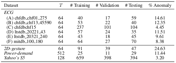
각 dataset의 dimension

Dataset	Dimension
ECG	bivariate
2D-gesture	bivariate
Power-demand	univariate
Yahoo's S5 Webscope	univariate

* 3개 이상의 multivariate time series를 사용한 추가 실험이 존재했으면 좀 더 다른 비교군들과 비교하기 좋았을 것 같음