Multivariate Time-series Anomaly Detection via Graph Attention Network (a.k.a MTAD-GAT)
Multivariate Time-series Anomaly Detection via Graph Attention Network
2020 IEEE International Conference on Data Mining (ICDM)
Introduction
이전의 방법들의 한계점 : 시계열 간의 상관관계를 고려하지 않아 False Positive가 탐지 됨
실제 데이터 수집 상황은 multivariate
때문에 univariate time sereis의 이상읕 탐지
하는 것은 해당 시스템의 정상 작동 여부를 판단하기에 어려움이 있음
한 시계열이 변화가 바로 시스템 오류를 의미하지 않을 수 있음
➞ 시스템을 구성하고 있는 각 시계열 간의 상관관계를 확인하는 것이 필요함
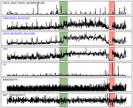
green : noraml / red : abnormal
초록색 영역의 2,3번 시계열 값이 갑작스럽게 증가
→ 이전의 방법들(주로 point-wise)을 사용하면 이상치로 판단할 것
→ 두 시계열의 변화 양상이 유사 : 정상 현상임
→ 시계열 간의 상관관계를 고려했을 때 두 시계열은 정상이며, 시게열 간의 상관관계를 고려하여 이상치를 탐지하는 것이 유의미 함
- EncDec-AD(ICML 2016)
LSTM Encoder-Decoder, reconstruction error - telemanom(KDD 2018)
LSTM based prediction - OmniAnomaly(KDD 2019)
stochastic recurrent nerural network, 데이터 분포를 모델링 해서 정상 패턴을 탐지
본 논문에서
1. 다변량 시계열에 존재하는 각 단변량 시계열 간의 상관관계를 포함하는 모델
2. 각 시계열 내의 temporal dependency를 반영하는 모델
을 만족하는 Multivariate Time-series Anomaly Detection via Graph Attention Network(MTAD-GAT)를 제안하고자 함
Methodology
basic structures
- 2개의 graph layer 사용
- feature-oriented : 각 시계열 간 인과관계 탐지
- time-oriendted : temporal dependency 탐지
-
2개의 모델을 함께 학습
-
forecasting based model
: focuse on single time stamp prediction -
reconstruction based model
: learn a latent representation of the entire time series
-
다변량 시계열은 단변량 시계열로 형성되어 있음
각 시계열 단위로 이상치를 탐지하는 것을 목표로 함
2개의 graph attention network를 parallel하게 쌓아 inter-feature correlation과 temporal dependency를 모델링
long-term dependency를 해결하기 위해 GRU(Gated Recurrent Unit)를 사용
notation
- : multivariate time-series input
- : num of timestamp(window length)
- : num of dimensions
- : label
는 timestamp가 anomaly인지 normal인지 나타냄 - : feature vector of each node
architecture
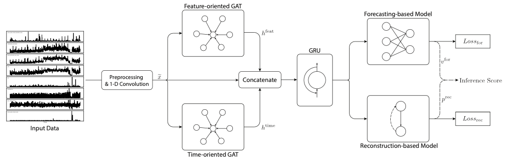
출처 : MTAD-GAT paper
-
Preprocessing & 1-D Convolution
-
normalization(MinMax) → train and test
-
cleaning
prediction and reconstruction based model은 noise에 민감
training set에 Spectral Residual 적용하여 이상치가 존재하는 time stamp 주변을 normal value로 대체
SR-CNN(KDD'19), SR(CVPR'07)
SR : target의 spectrum에서 average spectrum을 빼면 target의 특징만 남음 → anomaly detection에서는 이상치 부분이 남아 있을 것training 과정에서 깔끔한 normal data만 학습하기 위해 cleaning을 진행했을 것으로 생각함
-
feature extraction
각 시계열은 high-level feature extraction을 위해 1-D convolution 사용
convolution을 적용하는 것은 time window 내의 local feature 추출에 효과적
시간 순서 유지 & window 내의 정보를 함께 고려하여 embedding
-
- Graph Attention
graph layer → node 간의 relationship을 modeling
,
attention score , : node 의 adjacent node 수
GAT output , : activation function(sigmoid)
-
Feature-oriented GAT
multivariate time-series의 각 time-series의 상관성에 대한 사전 정보가 없음
→ complete graph(서로 다른 vertex 사이에 한 개 이상의 edge가 존재)를 가정
각 시계열은 node, 시계열 사이의 relationship은 edg로 표현
→ 모든 시계열이 서로 관련되어 있다고 가정
feature oriented GAT output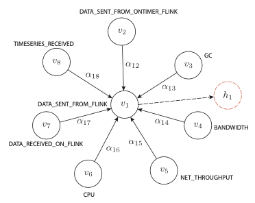 feature-oriented attention layer
: final output
-
Time-oriented GAT
temporal dependency를 capture하는 목적
sliding window 내의 timestamps는 complete graph로 가정
node 는 timestamp 시점의 각 dimension의 feature로 표현됨
-
layer's final output
feature-oriendted GAT layer:
time-oriented GAT layer :
after preprocessing data :
⇨ 3개의 output vector를 concat
는 GRU의 input으로 사용
서로 다른 information을 고려하여 학습하기 위함
- Joint Optimization
본 논문에서는 forecasting and reconstruction models을 함께 사용하여 각 모델 보완
각 model의 loss를 동시에 업데이트 시키는 것을 목적으로 함
-
forecasting-based model
three fully-connected layers 사용
next timestamp의 value를 예측
-
reconstruction-based model
VAE를 사용
latent representation 의 주변 데이터 분포 학습을 목표로 함
time series values를 variable로 취급하여시계열 값을 변수로 취급함으로써 VAE 모델은 전체 시계열의 데이터 분포를 캡처할 수 있습니다.
-
Score
: the number of features\
: a hyper-parameter to combine the forecasting-based error and the reconstrution-based probability
-
Experiments
Datasets
- SMAP (Soil Moisture Active Passice satellite)
- MSL (Mars Science Laboratory rover)
- Original dataset
Setting
- window size
- ; a grid search on the validation set(from 0.4 to 1.0)
- epochs : 100
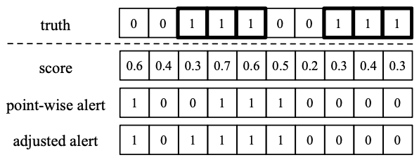
anomaly or not
보통 각각 point를 신경 쓰기 어렵고, 모든 anomaly point를 탐지하는 것은 어려움이 있음
따라서 아래 그림과 같은 조정된 판단 기준을 사용
- point : 0.5 이상 → anomaly
- adjusted strategy → segment 내에서 anomaly와 인접한 point도 anomaly로 판단
Unsupervised Anomaly Detection via Variational Auto-Encoder for Seasonal KPIs in Web Applications(WWW'18)
Conclusion
- inter and intra time seires relationship
- time seires 간의 관계 파악 → root cause 파악 가능
- feature 간 관계에 대한 사전 지식 없이 실험 → 사전 지식이 포함되면 성능 향상 가능성 존재
