
머신러닝·딥러닝 문제해결 전략 책을 읽으면서
Kaggle 경진대회 코드와 문제해결 전략을 정리한 글
6장 자전거 대여 수요 예측 경진대회 - 성능 개선
성능 개선Ⅰ : 릿지 회귀 모델
- 릿지(ridge) 회귀 모델 : L2 규제를 적용한 선형 회귀 모델
- 규제(regularization) : 모델이 훈련 데이터에 과대적합(overfitting)되지 않도록 해주는 방법
- 릿지 회귀 모델은 성능이 좋은 편은 아니고 단순 선형 회귀 모델보다 과대적합이 적은 모델 정도임
import pandas as pd
# 데이터 경로
data_path = '/kaggle/input/bike-sharing-demand/'

train = pd.read_csv(data_path + 'train.csv')
test = pd.read_csv(data_path + 'test.csv')
submission = pd.read_csv(data_path + 'sampleSubmission.csv')
피처 엔지니어링
- 피처 엔지니어링은 데이터를 변환하는 작업
- 이 변환을 훈련 데이터와 테스트 데이터에 공통으로 반영해야 하기 때문에, 피처 엔지니어링 전에 두 데이터를 합쳤다가 다 끝나면 나눠줌
- 데이터를 합치기 전에 훈련 데이터에서 이상치 하나를 제거하고 시작
이상치 제거
- 앞서 포인트 플롯에서 확인한 결과 훈련 데이터에서 weather가 4인 데이터(폭우, 폭설이 내리는 날 저녁 6시에 대여)는 이상치였고 이를 제거하도록 함
# 훈련 데이터에서 weather가 4가 아닌 데이터만 추출
train = train[train['weather'] != 4]
데이터 합치기
- 훈련 데이터와 테스트 데이터에 같은 피처 엔지니어링을 적용하기 위해 두 데이터를 하나로 합치기
- 판다스의 concat() 함수를 사용하면 축을 따라 DataFrame을 이어붙일 수 있음
훈련 데이터 : 10,886 행
테스트 데이터 : 6,493 행
총 데이터 : 17,379 행
weather가 4인 데이터를 제거했으니(1개 있음) 최종적으로 17,378행
all_data_temp = pd.concat([train, test])
all_data_temp| datetime | season | holiday | workingday | weather | temp | atemp | humidity | windspeed | casual | registered | count | |
|---|---|---|---|---|---|---|---|---|---|---|---|---|
| 0 | 2011-01-01 00:00:00 | 1 | 0 | 0 | 1 | 9.84 | 14.395 | 81 | 0.0000 | 3.0 | 13.0 | 16.0 |
| 1 | 2011-01-01 01:00:00 | 1 | 0 | 0 | 1 | 9.02 | 13.635 | 80 | 0.0000 | 8.0 | 32.0 | 40.0 |
| 2 | 2011-01-01 02:00:00 | 1 | 0 | 0 | 1 | 9.02 | 13.635 | 80 | 0.0000 | 5.0 | 27.0 | 32.0 |
| 3 | 2011-01-01 03:00:00 | 1 | 0 | 0 | 1 | 9.84 | 14.395 | 75 | 0.0000 | 3.0 | 10.0 | 13.0 |
| 4 | 2011-01-01 04:00:00 | 1 | 0 | 0 | 1 | 9.84 | 14.395 | 75 | 0.0000 | 0.0 | 1.0 | 1.0 |
| ... | ... | ... | ... | ... | ... | ... | ... | ... | ... | ... | ... | ... |
| 6488 | 2012-12-31 19:00:00 | 1 | 0 | 1 | 2 | 10.66 | 12.880 | 60 | 11.0014 | NaN | NaN | NaN |
| 6489 | 2012-12-31 20:00:00 | 1 | 0 | 1 | 2 | 10.66 | 12.880 | 60 | 11.0014 | NaN | NaN | NaN |
| 6490 | 2012-12-31 21:00:00 | 1 | 0 | 1 | 1 | 10.66 | 12.880 | 60 | 11.0014 | NaN | NaN | NaN |
| 6491 | 2012-12-31 22:00:00 | 1 | 0 | 1 | 1 | 10.66 | 13.635 | 56 | 8.9981 | NaN | NaN | NaN |
| 6492 | 2012-12-31 23:00:00 | 1 | 0 | 1 | 1 | 10.66 | 13.635 | 65 | 8.9981 | NaN | NaN | NaN |
17378 rows × 12 columns
# 원래 데이터의 인덱스를 무시하고 이어붙이려면 ignore_index=True를 전달
all_data = pd.concat([train, test], ignore_index=True)
all_data| datetime | season | holiday | workingday | weather | temp | atemp | humidity | windspeed | casual | registered | count | |
|---|---|---|---|---|---|---|---|---|---|---|---|---|
| 0 | 2011-01-01 00:00:00 | 1 | 0 | 0 | 1 | 9.84 | 14.395 | 81 | 0.0000 | 3.0 | 13.0 | 16.0 |
| 1 | 2011-01-01 01:00:00 | 1 | 0 | 0 | 1 | 9.02 | 13.635 | 80 | 0.0000 | 8.0 | 32.0 | 40.0 |
| 2 | 2011-01-01 02:00:00 | 1 | 0 | 0 | 1 | 9.02 | 13.635 | 80 | 0.0000 | 5.0 | 27.0 | 32.0 |
| 3 | 2011-01-01 03:00:00 | 1 | 0 | 0 | 1 | 9.84 | 14.395 | 75 | 0.0000 | 3.0 | 10.0 | 13.0 |
| 4 | 2011-01-01 04:00:00 | 1 | 0 | 0 | 1 | 9.84 | 14.395 | 75 | 0.0000 | 0.0 | 1.0 | 1.0 |
| ... | ... | ... | ... | ... | ... | ... | ... | ... | ... | ... | ... | ... |
| 17373 | 2012-12-31 19:00:00 | 1 | 0 | 1 | 2 | 10.66 | 12.880 | 60 | 11.0014 | NaN | NaN | NaN |
| 17374 | 2012-12-31 20:00:00 | 1 | 0 | 1 | 2 | 10.66 | 12.880 | 60 | 11.0014 | NaN | NaN | NaN |
| 17375 | 2012-12-31 21:00:00 | 1 | 0 | 1 | 1 | 10.66 | 12.880 | 60 | 11.0014 | NaN | NaN | NaN |
| 17376 | 2012-12-31 22:00:00 | 1 | 0 | 1 | 1 | 10.66 | 13.635 | 56 | 8.9981 | NaN | NaN | NaN |
| 17377 | 2012-12-31 23:00:00 | 1 | 0 | 1 | 1 | 10.66 | 13.635 | 65 | 8.9981 | NaN | NaN | NaN |
17378 rows × 12 columns
파생 피처(변수) 추가
from datetime import datetime

# 날짜 피처 생성
all_data['date'] = all_data['datetime'].apply(lambda x: x.split()[0])
# 연도 피처 생성
all_data['year'] = all_data['datetime'].apply(lambda x: x.split()[0].split('-')[0])
# 월 피처 생성
all_data['month'] = all_data['datetime'].apply(lambda x: x.split()[0].split('-')[1])
# 시 피처 생성
all_data['hour'] = all_data['datetime'].apply(lambda x: x.split()[1].split(':')[0])
# 요일 피처 생성
all_data['weekday'] = all_data['date'].apply(lambda dateString: datetime.strptime(dateString, '%Y-%m-%d').weekday())- 훈련 데이터는 매달 1일부터 19일까지의 기록이고, 테스트 데이터는 매달 20일부터 월말까지의 기록
- 그러므로 대여 수량을 예측할 때 일(day) 피처는 사용할 필요가 없음
- minute와 second 피처도 모든 기록에서 값이 같으므로 예측에 사용할 필요가 없음
- 그래서 day, minute, second는 피처로 생성하지 않았음
필요 없는 피처 제거
- casual과 registered 피처는 테스트 데이터에 없는 피처이므로 제거
- datetime 피처는 인덱스 역할이고 date 피처가 갖는 정보들은 다른 피처들(year, month, day)에도 담겨 있기 때문에 datetime과 date 피처도 필요 없음
- season 피처가 month의 대분류 성격이라서 month 피처도 제거
- windspeed 피처도 타깃값과 상관관계가 약하므로 제거
drop_features = ['casual', 'registered', 'datetime', 'date', 'windspeed', 'month']

all_data = all_data.drop(drop_features, axis=1)- 필요 없는 피처를 제거함으로써 모델링할 때 사용할 피처를 모두 선별
- 탐색적 데이터 분석에서 얻은 인사이트를 활용해 의미 있는 피처와 불필요한 피처를 구분
- 이러한 과정을 피처 선택이라고 함
피처 선택(feature selection) : 모델링 시 데이터의 특징을 잘 나타내는 주요 피처만 선택하는 작업
데이터 나누기
- 모든 피처 엔지니어링을 적용했으므로 훈련 데이터와 테스트 데이터를 다시 나누기
# 훈련 데이터와 테스트 데이터 나누기
X_train = all_data[~pd.isnull(all_data['count'])]   # 타깃값이 있으면 훈련 데이터
X_test = all_data[pd.isnull(all_data['count'])]     # 타깃값이 없으면 테스트 데이터

# 타깃값 count 제거
X_train = X_train.drop(['count'], axis=1)
X_test = X_test.drop(['count'], axis=1)

y = train['count']  # 타깃값
# 피처 엔지니어링 후의 훈련 데이터
X_train.head()| season | holiday | workingday | weather | temp | atemp | humidity | year | hour | weekday | |
|---|---|---|---|---|---|---|---|---|---|---|
| 0 | 1 | 0 | 0 | 1 | 9.84 | 14.395 | 81 | 2011 | 00 | 5 |
| 1 | 1 | 0 | 0 | 1 | 9.02 | 13.635 | 80 | 2011 | 01 | 5 |
| 2 | 1 | 0 | 0 | 1 | 9.02 | 13.635 | 80 | 2011 | 02 | 5 |
| 3 | 1 | 0 | 0 | 1 | 9.84 | 14.395 | 75 | 2011 | 03 | 5 |
| 4 | 1 | 0 | 0 | 1 | 9.84 | 14.395 | 75 | 2011 | 04 | 5 |
평가지표 계산 함수 작성
- 훈련이란 어떠한 능력을 개선하기 위해 배우거나 단련하는 행위
- 따라서 훈련이 제대로 이루어졌는지 확인하려면 대상 능력을 평가할 수단, 즉 평가지표가 필요함
- 그래서 본격적인 훈련에 앞서 본 경진대회 평가지표인 RMSLE를 계산하는 함수 만들기
import numpy as np

def rmsle(y_true, y_pred, convertExp=True):
    # 지수변환
    if convertExp:
        y_true = np.exp(y_true)
        y_pred = np.exp(y_pred)

    # 로그변환 후 결측값을 0으로 변환
    log_true = np.nan_to_num(np.log(y_true+1))
    log_pred = np.nan_to_num(np.log(y_pred+1))

    # RMSLE 계산
    output = np.sqrt(np.mean((log_true - log_pred)**2))
    return output
실제 타깃값 y_true와 예측값 y_pred를 인수로 전달하면 RMSLE 수치를 반환하는 함수
- convertExp는 입력 데이터를 지수변환할지를 정하는 파라미터
- 기본값인 convertExp=True를 전달하면 y_true와 y_pred를 지수변환
- 지수변환에는 넘파이 내장 함수인 exp() 이용
- 지수변환하는 이유는 타깃값으로 count가 아닌 log(count)를 사용하기 때문
- y_true와 y_pred를 로그변환하고 결측값은 0으로 변환
- np.log() 함수의 밑은 e
- np.nan_to_num() 함수는 NaN 결측값을 모두 0으로 바꾸는 기능을 함
하이퍼파라미터 최적화 (모델 훈련)
- '모델 훈련' 단계에서 그리드서치 기법을 사용
- 그리드서치(grid search)는 하이퍼파라미터를 격자(grid)처럼 촘촘하게 순회하며 최적의 하이퍼파라미터 값을 찾는 기법
- 각 하이퍼파라미터를 적용한 모델마다 교차 검증(cross-validation)하며 성능을 측정하여 최종적으로 성능이 가장 좋았을 때의 하이퍼파라미터 값을 찾아줌
- 교차 검증 평가점수는 보통 에러 값이기 때문에 낮을수록 좋음
모델 생성
# 릿지 모델 생성
from sklearn.linear_model import Ridge
from sklearn.model_selection import GridSearchCV
from sklearn import metrics

ridge_model = Ridge()
그리드서치 객체 생성
- 그리드서치는 '하이퍼파라미터의 값'을 바꿔가며 '모델'의 성능을 교차 검증으로 '평가'해 최적의 하이퍼파라미터 값을 찾아줌
- 그러므로 그리드서치 객체는 다음의 세 가지를 알고 있어야 함
- 비교 검증해볼 하이퍼파라미터 값 목록
- 대상 모델
- 교차 검증용 평가 수단(평가 함수)
- 릿지 모델은 규제를 적용한 회귀 모델인데, 릿지 모델에서 중요한 하이퍼파라미터는
alpha로, 값이 클수록 규제 강도가 커짐. 즉,alpha를 적당한 크기로 하면 과대적합 문제를 개선할 수 있음
# 하이퍼파라미터 값 목록
ridge_params = {'max_iter': [3000],
                'alpha': [0.1, 1, 2, 3, 4, 10, 30, 100, 200, 300, 400, 800, 900, 1000]}

# 교차 검증용 평가 함수(RMSLE 점수 계산)
rmsle_scorer = metrics.make_scorer(rmsle, greater_is_better=False)
# make_scorer는 평가지표 계산 함수와 평가지표 점수가 높으면 좋은지 여부 등을 인수로 받는 교차 검증용 평가 함수

# 그리드서치(with 릿지) 객체 생성
gridsearch_ridge_model = GridSearchCV(estimator=ridge_model,     # 릿지 모델
                                      param_grid=ridge_params,   # 하이퍼파라미터 값 목록
                                      scoring=rmsle_scorer,      # 평가지표
                                      cv=5)                      # 교차 검증 분할 수
그리드서치 객체를 생성하는 GridSearchCV()함수의 주요 파라미터
- estimator : 분류 및 회귀 모델
- param_grid : 딕셔너리 형태로 모델의 하이퍼파라미터명과 여러 하이퍼파라미터 값을 지정
- scoring : 평가지표. 사이킷런에서 기본적인 평가지표를 문자열 형태로 제공함. 사이킷런에서 제공하는 평가지표를 사용하지 않고 별도로 만든 평가지표를 사용해도 됨.
- cv : 교차 검증 분할 개수 (기본값은 5)
그리드서치 수행
log_y = np.log(y)  # 타깃값 로그변환
gridsearch_ridge_model.fit(X_train, log_y)  # 훈련(그리드서치)
GridSearchCV(cv=5, estimator=Ridge(),
param_grid={'alpha': [0.1, 1, 2, 3, 4, 10, 30, 100, 200, 300, 400,
800, 900, 1000],
'max_iter': [3000]},
scoring=make_scorer(rmsle, greater_is_better=False))fit()을 실행하면 객체 생성 시 paramgrid에 전달된 값들을 순회하면서 교차 검증으로 평가지표 점수를 계산함. 이때 가장 좋은 성능을 보인 값을 **best_params 속성에 저장하며, 이 최적 값으로 훈련한 모델(최적 예측기)을 bestestimator** 속성에 저장함.
print('최적 하이퍼파라미터 :', gridsearch_ridge_model.best_params_)최적 하이퍼파라미터 : {'alpha': 0.1, 'max_iter': 3000}성능 검증
- 그리드서치 객체의 bestestimator 속성에 저장된 모델로 성능 검증 수행
# 예측
preds = gridsearch_ridge_model.best_estimator_.predict(X_train)

# 평가
print(f'릿지 회귀 RMSLE 값 : {rmsle(log_y, preds, True):.4f}')
릿지 회귀 RMSLE 값 : 1.0205참 값(log_y)와 예측값(preds) 사이의 RMSLE는 1.02로, 선형 회귀 모델의 결과와 다르지 않음
성능 개선Ⅱ : 라쏘 회귀 모델
- 라쏘(lasso) 회귀 모델 : L1 규제를 적용한 선형 회귀 모델
- 규제(regularization) : 모델이 훈련 데이터에 과대적합(overfitting)되지 않도록 해주는 방법
- 릿지 회귀 모델과 마찬가지로 라쏘 회귀 모델도 성능이 좋은 편은 아님
하이퍼파라미터 최적화 (모델 훈련)
- rmsle_scorer 함수는 릿지 회귀 때 정의한 것을 재활용하였고 릿지 회귀와 마찬가지로
alpha는 규제 강도를 조정하는 파라미터
from sklearn.linear_model import Lasso

# 모델 생성
lasso_model = Lasso()

# 하이퍼파라미터 값 목록
lasso_alpha = 1/np.array([0.1,1,2,3,4,10,30,100,200,300,400,800,900])
lasso_params = {'max_iter':[3000], 'alpha':lasso_alpha}

# 그리드서치(with 라쏘) 객체 생성
gridsearch_lasso_model = GridSearchCV(estimator=lasso_model,
                                      param_grid=lasso_params,
                                      scoring=rmsle_scorer,
                                      cv=5)

# 그리드서치 수행
log_y = np.log(y)
gridsearch_lasso_model.fit(X_train, log_y)

print('최적 하이퍼파라미터 :', gridsearch_lasso_model.best_params_)
최적 하이퍼파라미터 : {'alpha': 0.00125, 'max_iter': 3000}성능 검증
# 예측
preds = gridsearch_lasso_model.best_estimator_.predict(X_train)

# 평가
print(f'라쏘 회귀 RMSLE 값: {rmsle(log_y, preds, True):.4f}')
라쏘 회귀 RMSLE 값: 1.0205결과를 보면 RMSLE 값은 1.02로 여전히 개선되지 않음
성능 개선Ⅲ : 랜덤 포레스트 회귀 모델
- 랜덤 포레스트(random forest) 회귀는 간단히 생각하면 훈련 데이터를 랜덤하게 샘플링한 모델 n개를 각각 훈련하여 결과를 평균하는 방법
하이퍼파라미터 최적화 (모델 훈련)
from sklearn.ensemble import RandomForestRegressor

# 모델 생성
randomforest_model = RandomForestRegressor()

# 그리드서치 객체 생성
rf_params = {'random_state':[42], 'n_estimators':[100, 120, 140]}
gridsearch_random_forest_model = GridSearchCV(estimator=randomforest_model,
                                              param_grid=rf_params,
                                              scoring=rmsle_scorer,
                                              cv=5)

# 그리드서치 수행
log_y = np.log(y)
gridsearch_random_forest_model.fit(X_train, log_y)
print('최적 하이퍼파라미터 :', gridsearch_random_forest_model.best_params_)
최적 하이퍼파라미터 : {'n_estimators': 140, 'random_state': 42}- random_state는 랜덤 시드값으로, 값을 명시하면 코드를 다시 실행해도 같은 결과를 얻을 수 있음
- n_estimators는 랜덤 포레스트를 구성하는 결정 트리 개수를 의미
모델 성능 검증
# 예측
preds = gridsearch_random_forest_model.best_estimator_.predict(X_train)

# 평가
print(f'랜덤 포레스트 회귀 RMSLE 값 : {rmsle(log_y, preds, True):.4f}')
랜덤 포레스트 회귀 RMSLE 값 : 0.1126랜덤 포레스트 회귀 모델을 사용하니 RMSLE 값이 큰 폭으로 개선됨
선형 회귀, 릿지 회귀, 라쏘 회귀 모델의 RMSLE 값은 모두 1.02인 반면
랜덤 포레스트 회귀 모델은 0.11 → 네 모델 중 성능이 가장 좋은 모델
예측 및 결과 제출
- 성능이 가장 좋은 모델의 예측 결과를 제출 → 검증 결과 랜덤 포레스트 회귀 모델의 성능이 가장 좋았음
- 성능 측정을 훈련 데이터로 했기 때문에 테스트 데이터에서도 성능이 좋다고 보장할 수는 없음
- 다행히 본 경진대회는 훈련 데이터와 테스트 데이터의 분포가 비슷함
- 두 데이터 분포가 비슷하면 과대적합 문제가 상대적으로 적기 때문에 훈련 데이터에서 성능이 좋다면 테스트 데이터에서도 좋을 가능성이 큼
훈련 데이터 타깃값과 테스트 데이터 타깃 예측값의 분포
import seaborn as sns
import matplotlib.pyplot as plt

randomforest_preds = gridsearch_random_forest_model.best_estimator_.predict(X_test)

figure, axes = plt.subplots(ncols=2)
figure.set_size_inches(10, 4)

sns.histplot(y, bins=50, ax=axes[0])
axes[0].set_title('Train Data Distribution')
sns.histplot(np.exp(randomforest_preds), bins=50, ax=axes[1])
axes[1].set_title('Predicted Test Data Distribution')
Text(0.5, 1.0, 'Predicted Test Data Distribution')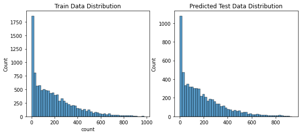
submission['count'] = np.exp(randomforest_preds)  # 지수변환
submission.to_csv('submission.csv', index=False)
핵심 요약
- 캐글 경진대회 프로세스는 크게 '경진대회 이해' → '탐색적 데이터 분석' → '베이스라인 모델' → '성능 개선' 순으로 진행되며 일반적인 머신러닝/딥러닝 문제를 해결할 때도 그대로 적용할 수 있음
- 경진대회 이해 단계에서는 대회의 취지와 문제 유형을 정확히 파악하고, 평가지표를 확인함
- 탐색적 데이터 분석 단계에서는 시각화를 포함한 각종 기법을 동원해 데이터를 분석하여, 피처 엔지니어링과 모델링 전략을 수립.
- 베이스라인 모델 단계에서는 본격적인 최적화에 앞서 기본 모델을 제작. 유사한 문제를 풀 때 업계에서 흔히 쓰는 모델이나 직관적으로 떠오르는 모델을 선택함.
- 성능 개선 단계에서는 베이스라인 모델보다 나은 성능을 목표로 각종 최적화를 진행.
- 타깃값이 정규분포에 가까울수록 회귀 모델의 성능이 좋음. 한쪽으로 치우친 타깃값은 로그변환하면 정규분포에 가까워지고, 결괏값을 지수변환하면 원래 타깃값 형태로 복원됨(타깃값 변환).
- 훈련 데이터에서 이상치를 제거하면 일반화 성능이 높아질 수 있음(이상치 제거).
- 기존 피처를 분해/조합하여 모델링에 도움되는 새로운 피처를 추가할 수 있음(파생 피처 추가).
- 반대로 불필요한 피처를 제거해주면 성능도 좋아지고, 훈련 속도도 빨라짐(피처 제거).
- 선형 회귀, 릿지, 라쏘 모델은 회귀 문제를 푸는 대표적인 모델이지만, 너무 기본적이라 실전에서 단독으로 최상의 성능을 기대하기는 어려움.
- 랜덤 포레스트 회귀 모델은 여러 모델을 묶어 (대체로) 더 나은 성능을 이끌어내는 간단하고 유용한 기법.
- 그리드서치는 교차 검증으로 최적의 하이퍼파라미터 값을 찾아주는 기법.
