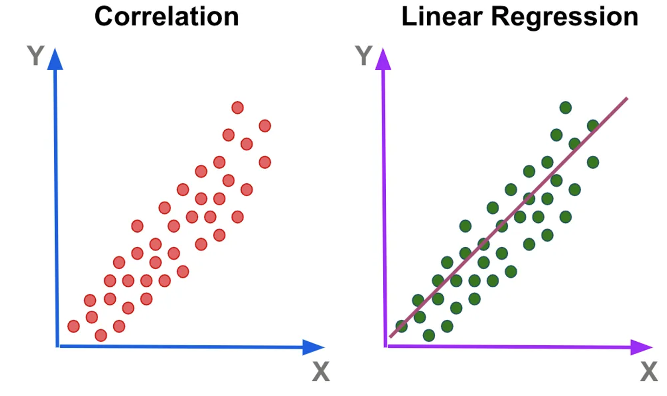
Linear Regression

Linear regression → 연속적인 값을 추정

Normal equation → 선형대수학적으로 최적화된 해를 구함

Gradient descent → 값의 근사 (미분을 이용)

What is Linear Regression

input → model → output

(trainset) (prediction)

이때, cost를 최소화 하는 방향으로 학습을 시킴 → model에 대한 개선

Linear model

input (vector) → linear model (linear regression) → output (real number, scalar)

• $\hat{y}$은 실제 $y$에 대한 예측된 변수

• $n$은 feature의 수, $n$차원, input에 들어있는 값의 수

• $x_i$의 경우 $i$번째 feature 값

• $\theta_j$의 경우 $j$번째 model parameter, 각 feature에 대한 weight $\theta_1, \theta_2, ..., \theta_n$에 bias인 $\theta_0$을 더한 값

• $\Theta$는 model의 parameter vector을 나타냄. model을 기술하는데 필요한 parameter

• $x$의 경우 feature vector이다. 이는 input이다. $x_0$의 경우 1이며, 이는 bias를 위한 값이다.

$\hat{y} = \theta_0 + \theta_1x_1$

1. $\theta = \begin{bmatrix} 0 \\ 1 \\ \end{bmatrix}$
2. $\theta = \begin{bmatrix} -1 \\ 2 \\ \end{bmatrix}$

이 때, bias $\theta$에 따라 직선의 기울기가 달라진다. parameter $\theta_0$과 $\theta_1$을 조정하여 주어진 data를 가장 잘 설명하는 parameter $\theta$를 구한다.

parameter $\theta$가 결정되는 순간 예측값은 하나의 직선으로 표현된다 → 우리의 prediction을 모든 영역에 대해 표현한다

실제값과 예측값의 차이를 error라고 할 때, error = $y - \hat{y}$로 표현할 수 있다.

이때, error의 값은 거리값이므로 $(y - \hat{y})^2$로 제곱을 취하고, 이는 항상 양수값이다.

$i$ $i$$error^{(i)} = (y^{(i)} - \hat{y}^{(i)})^2$로 표현할 수 있고, 각 sample에 대한 error을 정의할 수 있다.

$\sum_{i=1}^{5}error^{(i)2} = \sum_{i=1}^{5}(y^{(i)} - \hat{y}^{(i)})^2$을 위의 1번 model과 2번 model에 대해 구할 수 있다.

1번 model의 $error^2$의 값을 20, 2번 model의 $error^2$의 값을 100이라 할 때, 주어진 data를 잘 설명하는 model은 1번 model이라고 할 수 있다.

Cost function

linear regression model에 대한 parameter은 어떻게 찾는가?

model을 training한다는 뜻은 적합한 주어진 training set에 가장 적합한 model을 찾아냄을 의미한다.

가장 먼저 현재 주어진 데이터에 대해 model이 얼마나 fit한지 판단해야 한다

regression problem에 사용되는 measure, error index, cost function은 다음과 같다

여기서 $\Theta^Tx^{(i)} = \hat{y}^{(i)}$이다.

RMSE: Root Mean Of Squared error

MSE: Mean Of Squared error

SSE: Sum Of Squared error

RMSE, MSE, SSE를 최소로 만드는 argument의 해는 동일하다

Design matrix

• regressor matrix, model matrix, data matrix
• model은 $\hat{y} = \Theta^Tx$
• training dataset은 $(x^{(1)}, y^{(1)}), \space (x^{(2)}, y^{(2)}), \space (x^{(3)}, \space y^{(3)}), \space ..., \space (x^{(m)}, y^{(m)})$
• model prediction은 $(\hat{y}^{(1)} = \Theta^Tx^{(1)}), \space (\hat{y}^{(2)} = \Theta^Tx^{(2)}), \space(\hat{y}^{(3)} = \Theta^Tx^{(3)}), \space... \space , \space (\hat{y}^{(m)} = \Theta^Tx^{(m)}), \space$
• SSE는 $(y^{(1)} - \Theta^Tx^{(1)})^2 + (y^{(2)} - \Theta^Tx^{(2)})^2 + (y^{(3)} - \Theta^Tx^{(3)})^2 + ... + (y^{(m)} - \Theta^Tx^{(m)})^2$

이를 input $X = \begin{bmatrix} x^{(1)T} \\ x^{(2)T} \\ \vdots \\ x^{(m)T} \\ \end{bmatrix}$일 때, $\hat{y} = \begin{bmatrix} \hat{y}^{(1)} \\ \hat{y}^{(2)} \\ \vdots \\ \hat{y}^{(m)} \\ \end{bmatrix}$ = $X \cdot \Theta = \begin{bmatrix} x^{(1)T} \\ x^{(2)T} \\ \vdots \\ x^{(m)T} \\ \end{bmatrix} \cdot \Theta$로 표현할 수 있다.

$SSE(\Theta) = \sum_{i=1}^{m}(y^{(i)} - \Theta^Tx^{(i)})^2 \newline = \| y - \hat{y} \|^2_2 \newline = \| \begin{bmatrix} y^{(1)} \\ y^{(2)} \\ \vdots \\ y^{(m)} \\ \end{bmatrix} - \begin{bmatrix} \hat{y}^{(1)} \\ \hat{y}^{(2)} \\ \vdots \\ \hat{y}^{(m)} \\ \end{bmatrix} \|^2_2 \newline = \| \begin{bmatrix} y^{(1)} - \hat{y}^{(1)} \\ y^{(2)} - \hat{y}^{(2)} \\ \vdots \\ y^{(m)} - \hat{y}^{(m)} \\ \end{bmatrix} \|^2_2$

Design matrix에 대해 training dataset이 $m$개, feature vector $x$의 차원이 $n$일 때, $m$개의 sample을 row vector로 한 design matrix $X$로 표현할 수 있다.

Normal Equation

Geometric approach

Design matrix $X$의 각 열을 $\vec{x_j}$라고 하면

즉, $\hat{y}$는 $x_1, x_2, ..., x_n$이 생성하는 hyperplane인 span$\{1, x_1, ... ,x_n\}$ 상에 존재한다

Residual(잔차) 또는 error의 크기 $\|y-\hat{y}\|$을 최소화 하기 위해서는 위의 hyperplane과 error$y - \hat{y}$가 서로 수직이어야 한다

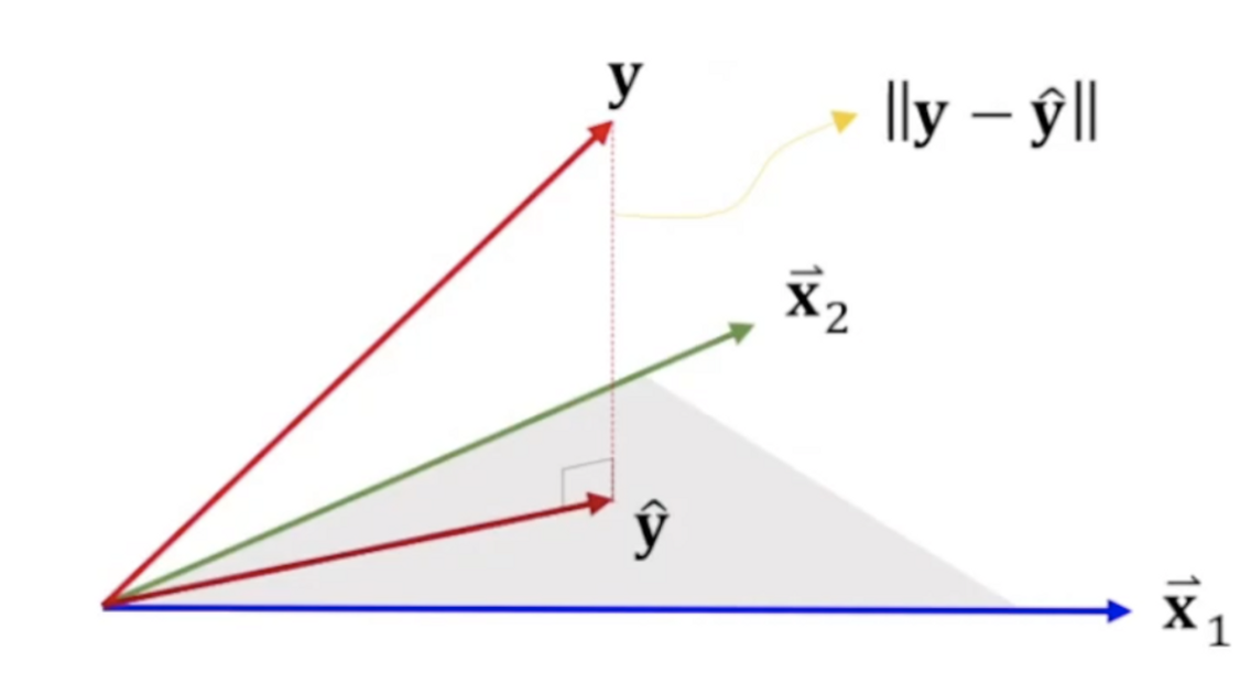
$\hat{y} = X \cdot \Theta \in span\{ x_1, x_2, ..., x_n \}$

$\hat{y}$는 $span$이라는 평면 위에 존재해야 한다. 이 때, $y$와 $\hat{y}$과의 거리가 가장 짧은 parameter $\theta$를 찾는다

이는 target인 $y$와 prediction인 $\hat{y}$가 수직에 위치할 때 거리가 가장 짧다

즉, $min \space \|y -\hat{y}\| \Leftrightarrow (y-\hat{y}) \perp span\{x_1, x_2, ..., x_n\}$이다.

즉, 모든 column vector에 대해서 $x^T_j \cdot (y-\hat{y})=0$이 성립해야 한다. → (수직이므로 내적값은 0)

전체 $m$의 sample에 대해 $X^T \cdot (y-X\theta) = 0 \Rightarrow X^TX\theta = X^Ty$이고, $\hat{\theta} = (X^TX)^{-1}X^Ty$이다

이는 $\hat{\theta} = (X^TX)^{-1}X^Ty \Leftrightarrow \hat{\theta} = arg \space min \space SSE(\theta)$를 유도한 것이다.

Analytic approach

Sum of squared error (SSE)에 대해

$\hat{y} = X\theta$를 사용하여

$SSE(\theta) = y^Ty - 2y^TX\theta + (X\theta)^T(X\theta) = y^Ty - 2y^TX\theta + \theta^TX^TX\theta$

$\frac{\partial SSE(\theta)}{\partial \theta} = 2(X^TX\theta - Xy) = 0 \Rightarrow X^TX\theta = X^Ty$

위 SSE를 미분하여 0이 나오는 값을 찾는다

따라서 우리는

$\hat{\theta} = (X^TX)^{-1}X^Ty$

$\hat{y} = X(X^TX)^{-1}X^Ty$

라는 normal equation을 얻을 수 있다.

Computational complexity

Normal equation의 계산

• Normal equation에 의한 예측치 $\hat{y} = X(X^TX)^{-1}X^Ty$
  
• $X \in R^{m \times n}$
• $X^TX \in R^{n \times n}$
• $(X^TX)^{-1}$의 계산 복잡도 = $O(n^{2.4})$ ~ $O(n^3)$
• Feature 수의 약 세제곱으로 계산 시간이 증가한다