[ML] Linear Regression 2

Gradient

어떤 미분에 대해서 gradient 라고 한다. 해당 경우에는 일반적인 scalar의 미분과는 다르다

vector → scalar의 경우 미분을 gradient라고 한다.

$f: R^n \rightarrow R$

$\nabla f: R^n \rightarrow R^n$ → Dimension이 동일함 (vector → vector)

$X \in R^2$

$f(X) = X^TX$

$f(x_1, x_2) = x_1^2+x_2^2$

$\nabla f(x_1, x_2) = \begin{bmatrix} \frac{\partial f(X)}{\partial x_1} \\ \frac{\partial f(X)}{\partial x_2} \\ \end{bmatrix}$

각 결과를 합쳐서 vector 하나로 만든다

$\because$ Gradient의 결과는 vector이어야 한다

ex) $f(x) = f(x_1, x_2, x_3) = x_1^2 + x_1x_2 + x_2x_3 + x_3^3$

해당 함수의 gradient $\nabla$$f(x)$는 다음과 같다

$\nabla f(X) = \begin{bmatrix} 2x_1 + x_2 \\ x_1 + x_3 \\ x_2 + 3x_3^2 \end{bmatrix}$이고, $R^3 \rightarrow R$이다.

즉, 3차원 vector에서 3차원 vector가 된다.

Gradient Descent

$f(x_1, x_2) = x_1^2 + x_2^2$, $R^2 \rightarrow R$

$\nabla f(x_1, x_2) = [2x_1 \space 2x_2]^T$으로 어떤 지점의 gradient vector을 구할 수 있다.

$f(X)$ 가 최소가 되는 $min$을 (근사적이고, iterative 하게) 찾는 여정을 gradient descent라고 할 수 있다.

$\eta$ 값을 조정하면서 하강법을 실행한다.

$\eta$: learning rate

ex) $f(x) = f(x_1, x_2, x_3) = x_1^2 + x_1x_2 + x_2x_3 + x_3^3$이고, $\eta = 0.1$일 때, 주어진 초기 위치 $\begin{bmatrix} 1 \space 1 \space 1\\ \end{bmatrix}^T$에서 한 번 갱신한 후의 위치 $x'$를 구하라

$\nabla f(x) = \begin{bmatrix} 2x_1+x_2 \\ x_1+x_3 \\ x_2+3x_3^2 \end{bmatrix}$이고, $\nabla f(\begin{bmatrix} 1 \\ 1 \\ 1 \end{bmatrix}) = \begin{bmatrix}3 \\ 2 \\ 4 \end{bmatrix}$이다.

따라서 $x' = x - \eta \nabla f(x) = {\begin{bmatrix} 1 \space 1 \space 1 \end{bmatrix}}^T - 0.1\begin{bmatrix} 3 \space 2 \space 4 \end{bmatrix}^T = \begin{bmatrix} 0.7 \\ 0.8 \\ 0.6 \end{bmatrix}$이다.

Gradient Decent는 다음과 같은 특징이 존재한다.

• 미분이 가능해야 한다.
• global minimum은 보장하지 못한다 → local minimum에 빠질 수 있다

Batch Gradient Descent

Linear regression model $\hat{y} = X\theta$가 존재한다고 하자.

$\hat{y} = X\theta$ ← 모든 sample에 대한 기술이 존재한다

즉, batch learning은 모든 sample에 대해서 학습을 시키는 방법이다 → parameter을 1번만 update한다

$J(\theta) = SSE(\theta) = \|y - X\theta\|^2 = \sum(y^{(n)} - \theta^TX^{(n)})^2$

이때, $J: R^n \rightarrow R$ 이다.

$\nabla_\theta J(\theta) = \frac{\partial}{\partial \theta} J(\theta) = 2X^T(X \theta - y)$

Batch gradient decent에서 $\frac{\partial}{\partial \theta}J(\theta) = 2X^T(X\theta-y)$를 전개하면 다음과 같다

$2[x^{(1)} \space x^{(2)} \space ... \space x^{(m)}] \begin{bmatrix} \theta^Tx^{(1)} - y^{(1)} \\ \theta^Tx^{(2)} - y^{(2)} \\ ... \\ \theta^Tx^{(m)} - y^{(m)} \end{bmatrix} = 2\sum_{i=1}^{m}x^{(i)}(\theta^Tx^{(i)} - y^{(i)})$

그러므로 해당 gradient vector의 j번째 component는
$\frac{\partial}{\partial \theta_j}J(\theta) = 2\sum_{i=1}^{m}x_{j}^{(i)}(\theta^Tx^{(i)} - y^{(i)})$이다

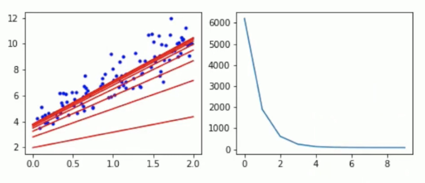
$\theta_0$부터 cost를 측정함, 해당 gradient를 통해 $\theta$를 업데이트함

parameter을 한 번 업데이트 할 경우 batch 전체에 대한 계산이 필요함. 따라서 dataset이 커지면 속도가 느려짐

Learning rate $\eta$ (hyperparameter) → 우리가 지정해야 하는 parameter

• $\eta$가 너무 작은 경우 시간이 오래 걸림
• $\eta$가 너무 큰 경우 최적해를 지나쳐 해를 찾지 못할 수도 있음

Learning schedule

Constant learning rate

• 보통 0.1, 0.01부터 시작하여 여러 가지 값으로 시험해보며 범위를 좁혀나감

Time-based decay

$\eta_0$: 학습률 초기값, $k$: hyperparameter, $t$: iteration

학습을 진행할 수록 $\eta$는 줄어드는 경항을 보임

Step decay

• 정해진 epoch마다 학습률을 줄이는 방법
  • 5 epoch마다 반으로, 20 epoch마다 1/10으로
  • Epoch: 훈련 데이터셋 전체를 모두 사용할 때 → 한 Epoch

Exponential decay

$\eta_0$: 학습률 초기값, $k$: hyperparameter, $t$: iteration

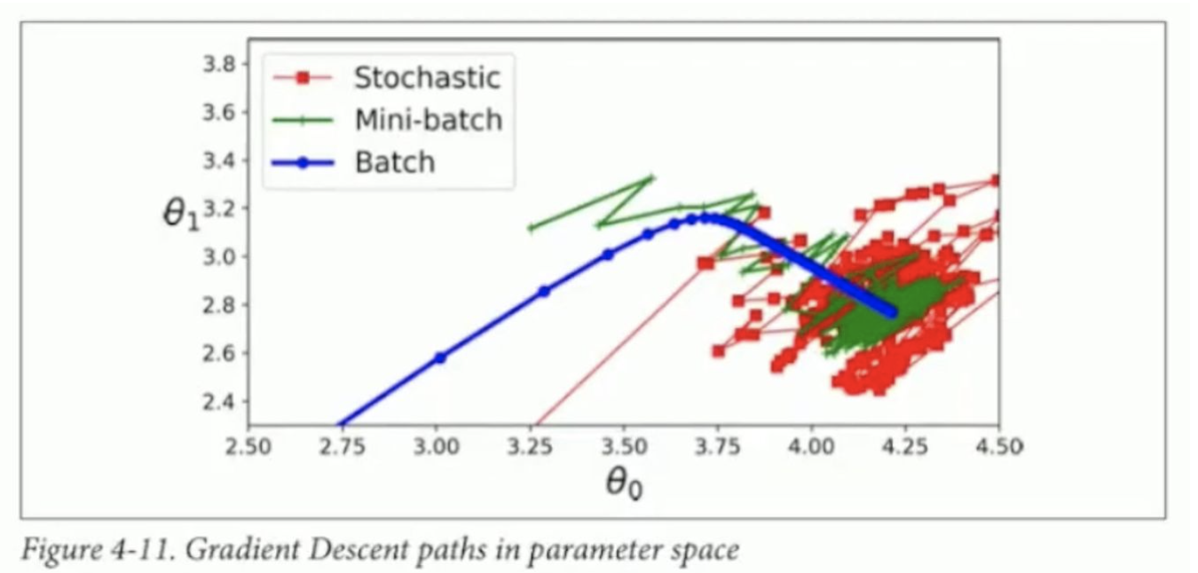
Stochastic Gradient Descent

무작위로 선택한 하나의 sample에 대해서 gradient를 계산해서 parameter를 update한다

대규모 데이터셋을 처리하는데 유리하며, 선택하는 사례의 무작위성으로 움직임이 불규칙적이다

Batch Gradient Descent에 비해 local optimum에서 쉽게 빠져나올 수 있다

최적해에 도달하지만 지속적으로 요동치며, Batch Gradient Descent와 마찬가지로 global optimum이라는 보장은 없다

Mini-batches Gradient Descent

훈련 데이터셋을 작은 크기의 무작위 부분 집합으로 나눠서 gradient를 구하는 방법

ex) 100,000개의 데이터 → (mini-batch size 100) x (1,000 mini-batches)

• 이 때의 epoch는 1,000당 1 epoch

Batch gradient descent와 Stochastic gradient descent의 절충안

Stochastic gradient descent보다 불규칙한 움직임이 덜하고, local minimum에서 빠져나오기가 상대적으로 어려움