Pandas
import pandas as pd
df = pd.read_csv('data/gapminder.tsv', sep='\t')
type(df)
df.head()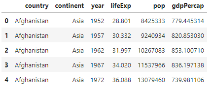
df.columns
Index(['country', 'continent', 'year', 'lifeExp', 'pop', 'gdpPercap'], dtype='object')

df.values
array([['Afghanistan', 'Asia', 1952, 28.801, 8425333, 779.4453145],
       ['Afghanistan', 'Asia', 1957, 30.332, 9240934, 820.8530296],
       ['Afghanistan', 'Asia', 1962, 31.997, 10267083, 853.10071],
       ...,
       ['Zimbabwe', 'Africa', 1997, 46.809, 11404948, 792.4499603],
       ['Zimbabwe', 'Africa', 2002, 39.989, 11926563, 672.0386227],
       ['Zimbabwe', 'Africa', 2007, 43.487, 12311143, 469.7092981]],
      dtype=object)

df.dtypes
country       object
continent     object
year           int64
lifeExp      float64
pop            int64
gdpPercap    float64
dtype: object

df.info()
<class 'pandas.core.frame.DataFrame'>
RangeIndex: 1704 entries, 0 to 1703
Data columns (total 6 columns):
 #   Column     Non-Null Count  Dtype
---  ------     --------------  -----
 0   country    1704 non-null   object
 1   continent  1704 non-null   object
 2   year       1704 non-null   int64
 3   lifeExp    1704 non-null   float64
 4   pop        1704 non-null   int64
 5   gdpPercap  1704 non-null   float64
dtypes: float64(2), int64(2), object(2)
memory usage: 80.0+ KB

df.loc[1:6, 'country':'year']
df.loc[[1,6], ['country','year']]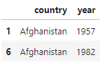
df.groupby('year')['lifeExp'].mean()
year
1952    49.057620
1957    51.507401
1962    53.609249
1967    55.678290
1972    57.647386
1977    59.570157
1982    61.533197
1987    63.212613
1992    64.160338
1997    65.014676
2002    65.694923
2007    67.007423
Name: lifeExp, dtype: float64

df.groupby('continent')['country'].nunique()
continent
Africa      52
Americas    25
Asia        33
Europe      30
Oceania      2
Name: country, dtype: int64
scientists = pd.DataFrame({
'Name': ['Rosaline Franklin', 'William Gosset'],
'Occupation': ['Chemist', 'Staristician'],
'Born': ['1920-07-25', '1876-06-13'],
'Died' : ['1958-04-16', '1937-10-16'],
'Age': [37, 61]}
)
print(scientists)
Name Occupation Born Died Age
0 Rosaline Franklin Chemist 1920-07-25 1958-04-16 37
1 William Gosset Staristician 1876-06-13 1937-10-16 61
df = pd.read_csv('data/scientists.csv')
df.values
array([['Rosaline Franklin', '1920-07-25', '1958-04-16', 37, 'Chemist'],
['William Gosset', '1876-06-13', '1937-10-16', 61, 'Statistician'],
['Florence Nightingale', '1820-05-12', '1910-08-13', 90, 'Nurse'],
['Marie Curie', '1867-11-07', '1934-07-04', 66, 'Chemist'],
['Rachel Carson', '1907-05-27', '1964-04-14', 56, 'Biologist'],
['John Snow', '1813-03-15', '1858-06-16', 45, 'Physician'],
['Alan Turing', '1912-06-23', '1954-06-07', 41,
'Computer Scientist'],
['Johann Gauss', '1777-04-30', '1855-02-23', 77, 'Mathematician']],
dtype=object)
df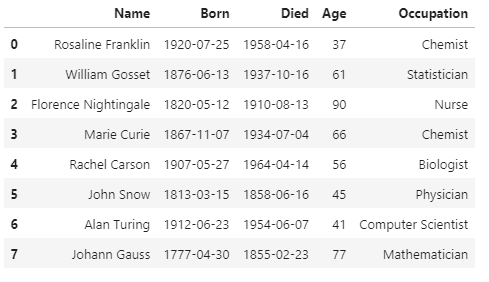
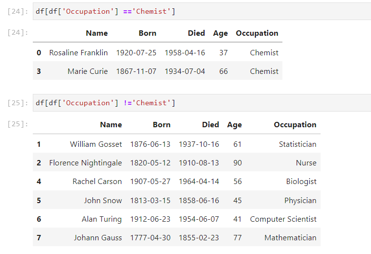
- 해당 값만 혹은 제외하고 추출하기
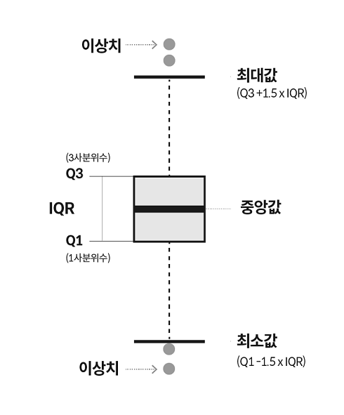
평균값과 사분위값
시각화
matplotlib, seaborn
import seaborn as sns
import matplotlib.pyplot as plt

df['dataset'].unique()

dataset1 = df[df['dataset']=='I']
dataset2 = df[df['dataset']=='II']
dataset3 = df[df['dataset']=='III']
dataset4 = df[df['dataset']=='IV']

plt.plot(dataset1['x'], dataset1['y'],'o')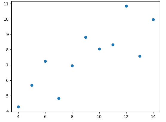
- 평균값은 같아도 실제 데이터분포는 다른 경우
fig = plt.figure()
a1 = fig.add_subplot(2,2,1)
a2 = fig.add_subplot(2,2,2)
a3 = fig.add_subplot(2,2,3)
a4 = fig.add_subplot(2,2,4)
a1.plot(dataset1['x'], dataset1['y'],'o')
a2.plot(dataset2['x'], dataset2['y'],'o')
a3.plot(dataset3['x'], dataset3['y'],'o')
a4.plot(dataset4['x'], dataset4['y'],'o')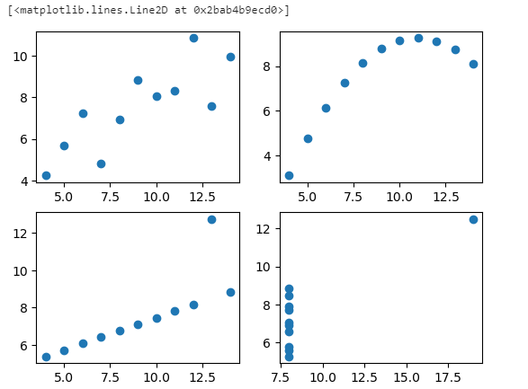
- 유형별 그래프
fig = plt.figure()
a1 = fig.add_subplot(1,1,1)
a1.hist(tips['total_bill'])
a1.set_title('Histgram of total bill')
a1.set_xlabel('Frequency')
a1.set_ylabel('total bill')
fig1 = plt.figure()
a1 = fig1.add_subplot(1,1,1)
a1.scatter(tips['total_bill'],tips['tip'])
a1.set_title('scatterplot of total bill vs tip')
a1.set_xlabel('total bill')
a1.set_ylabel('tip')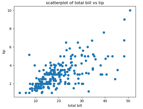
fig2 = plt.figure()
a1 = fig2.add_subplot(1,1,1)
a1.boxplot([tips[tips['sex'] == 'Female']['tip'],
            tips[tips['sex'] == 'Female']['tip']],
            labels = ['Female','Male'])
a1.set_title('boxplot of tips by sex')
a1.set_xlabel('sex')
a1.set_ylabel('tip')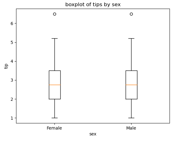

초보 개발자의 학습 저장용 블로그