1. 개요

Figure 1. Diffusion model 개요

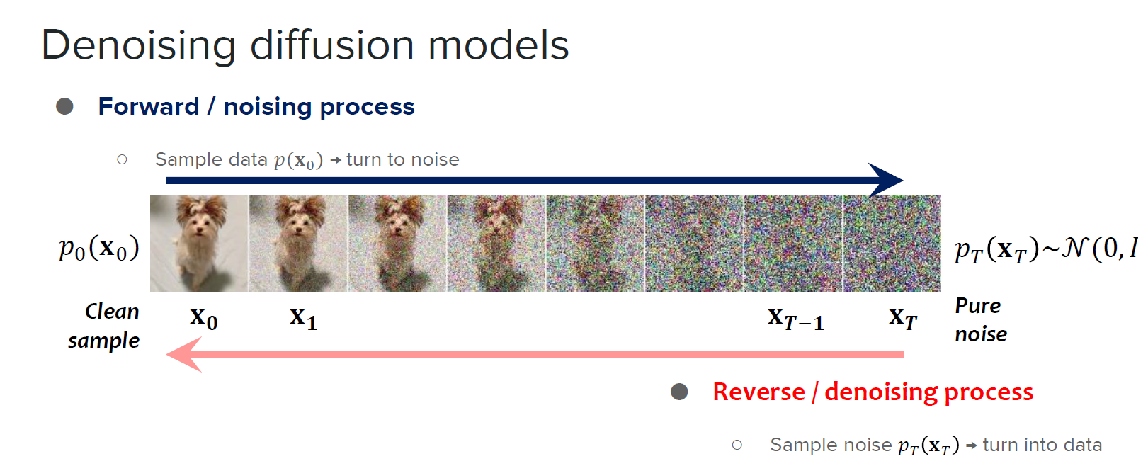
기본적인 diffusion model의 구조는 Figure 1과 같이 forward process와 reverse process로 설명될 수 있다. 먼저 forward process는 원본 이미지에 noise를 섞는 과정으로 보통 Gaussian noise가 사용되며, 위의 그림처럼 하나의 step마다 약간씩 노이즈를 추가해가면 결국 많은 step이 지났을 때 노이즈가 너무 많아져서 마치 Gaussian 분포에서 무작위로 픽셀값을 추출한 것만 같은 잡음 이미지가 된다.

다음으로 reverse process가 diffusion model에서 신경망 등을 통해 학습시키고자 하는 과정이며, 이는 forward process와는 반대로 노이즈가 섞여 있는 이미지가 입력되었을 때 해당 노이즈를 제거하는 과정이다. 따라서 forward process에서 몇 번의 step을 통해 최종적으로 완전한 잡음 이미지를 획득한 것처럼, reverse process에서는 잡음 이미지가 들어왔을 때, 몇 번의 step을 통해 완전히 노이즈를 걷어내어 깨끗한 이미지를 얻는 것이다.

이러한 diffusion model은 새로운 데이터를 생성하는 생성 모델에서 주로 사용되는데, 이것은 reverse process를 활용한 것으로, 학습이 잘 되어 있는 diffusion model에 무작위로 생성된 잡음 이미지를 입력하면, 학습 데이터셋에는 포함되어 있지 않은 잡음 이미지더라도 model이 나름대로 알아서 잡음을 걷어내고, 최종적으로는 어떠한 깨끗한 이미지가 생성된다. 어떤 이미지가 생성될 지는 입력되는 잡음 이미지에 따라 결정되며, 최근에는 conditional diffusion model을 통해 이미지를 어떻게 생성할 지 제어하기 위하여 잡음 이미지 뿐만 아니라 추가적인 정보(텍스트, 타겟 이미지 등)을 함께 입력하여 서비스를 제공하곤 한다.

이번 포스트에서는 diffusion model에 대한 식 유도와 함께, conditional diffusion model의 구조 등을 코드 예시와 함께 학습한다.

2. Diffusion model 수식

2.1. Forward Process

Forward process는 깨끗한 이미지에 몇 번의 step에 걸쳐 노이즈을 추가하는 과정이다. 이때, 처음의 깨끗한 데이터를 $x_0$, step을 $t$, 최종적인 잡음 이미지를 $x_T$라고 했을 때, Gaussian noise를 추가한다고 가정하면 다음과 같이 쓸 수 있다.

먼저 Markov 과정처럼 어떤 time step에서 노이즈를 추가할 때 바로 이전 step의 이미지에만 영향을 받으며, 이전 step의 값의 일부분만을 Gaussian의 평균값에 반영하여 유지시키고($\sqrt{1-\beta_t}\mathbf{x}_{t-1}$), 나머지 부분은 분산을 키워 무작위성을 높인다($\beta_t \mathbf{I}$). 이러한 과정을 $T$번 반복하면, 왼쪽과 같은 식이 되고, $T$가 충분히 크다면, 결국 평균은 0에 가까워지고, 분산은 커져서 완전한 잡음 데이터가 될 것이다.

이후 reverse process에서는 신경망을 통해 노이즈를 걷어내는 과정을 모델링하게되며, 이러한 신경망을 학습시키기 위해서 다양한 이미지에 위와 같은 forward process를 적용하여 time step 별로 노이즈가 섞이기 전 이미지와 섞인 후의 이미지를 수집하고 이를 학습데이터로 활용한다. 다만 성공적인 학습을 위해서는 이러한 데이터가 다량 필요하고, training loop를 한번 돌 때마다 이미지에 forward process를 처음부터 적용하여 데이터를 생성하면 시간이 많이 소요된다(만약 매우 큰 time step에서의 노이즈 섞인 이미지가 필요할 경우 forward process를 t=0부터 t=M까지 수행해야하기 때문). 하지만 수식을 약간 정리하면 임의의 time step에서의 노이즈 섞인 이미지를 바로 sampling할 수 있으며, 이는 학습 속도 개선에 큰 도움을 준다.

$\alpha_t = 1- \beta_t$, $\bar{\alpha}_t = \prod^t_{i=1}\alpha_i$라고 했을 때, 위와 같이 정의한 forward process에 대해서 임의의 time step의 데이터 $\mathbf{x}_t$에 대해서 다음과 같이 쓸 수 있다.

1번째 줄은 forward process의 정의식을 그대로 따른 것이며, 3번째 줄에서 4번째 줄로 넘어갈 때는 두 Gaussian distribution의 합을 생각하면 된다(두 Gaussian의 합이 만드는 분포의 평균과 분산은 각 분포의 평균의 합, 분산의 합으로 나타난다). 위의 식을 정리하면 다음과 같고, 임의의 time step에서의 노이즈 섞인 이미지를 만들기 위하여 굳이 forward process 전체를 수행하지 않아도 아래의 식을 통해서 바로 sampling 할 수 있음을 의미한다.

2.2. Reverse Process

Reverse process는 위의 forward process와는 반대로 입력 데이터의 노이즈를 제거하는 과정이다. 즉, forward process를 표현할 때는 $q(\mathbf{x}_t|\mathbf{x}_{t-1})$을 표현하는 방법을 찾았지만, reverse process에서는 $q(\mathbf{x}_{t-1}|\mathbf{x}_{t})$를 찾아야 한다. 이때, forward process야 입력 데이터에 Gaussian noise를 추가하며 진행되니 해당 정보를 이용하여 각각의 과정을 Gaussian distribution으로 표현할 수 있지만, reverse process는 어떤 분포로 나타나는 지 의문이다. Diffusion model의 논문(Sohl-Dickstein, Jascha, et al. "Deep unsupervised learning using nonequilibrium thermodynamics." International conference on machine learning. PMLR, 2015)에서 reverse process를 정의하고 있으며, (Feller, W. "On the theory of stochastic processes, with particular reference to applications." In Proceedings of the Berkeley Symposium on Mathematical Statistics and Probability. The Regents of the University of California, 1949.)에서 forward process가 Gaussian이나 binomial 이고 $\beta$가 작을 경우 reverse process 또한 forward process와 같은 형태의 분포로 나타남을 보였다고 한다. 즉 $q(\mathbf{x}_{t-1}|\mathbf{x}_{t})$ 또한 Gaussian 분포로 표현될 수 있다.

다만, $q(\mathbf{x}_{t-1}|\mathbf{x}_{t})$를 직접 계산하기는 어려워 다음과 같이 reverse process를 모델링하며, reverse process가 Gaussian 분포로 나타난다는 것을 알고 있기 때문에, 신경망을 통해 다음과 같이 Gaussian을 표현하는 평균과 분산을 모델링하도록 한다.

2.3. Loss Function

즉, $p_\theta$가 $q$와 유사해지도록 학습을 시켜야하고 최종적으로는 reverse process를 통해 원래의 데이터 $\mathbf{x}_0$를 복원해내야 한다. 이를 위한 loss function으로 다음과 같이 cross entropy를 사용하면 두 분포가 유사해지도록 학습시킬 수 있다.

하지만 VAE에서와 같은 논리로 loss function 안의 $p_\theta(\mathbf{x}_0)$는 직접적으로 계산하기가 어려운데, $p_\theta(\mathbf{x}_0)=\int p_\theta(\mathbf{x}_{0:T}) d\mathbf{x}_{1:T}$에서 이전 step에 해당하는 모든 $\mathbf{x}_{1:T}$에 대한 적분이 불가하기 때문이다. 따라서 VAE의 해법처럼 다음과 같이 lower bound(negative log를 사용할 경우 upper bound)를 이용하게 되며, 그 유도 방법에는 여러가지가 있을 수 있지만 여기서는 Jensen's inequality를 통한 방법을 소개한다(VAE 포스트도 참고).

위 처럼 유도된 negative log의 upper bound를 줄이면 자연스럽게 cross entropy 또한 줄어들게 된다. 이제 해당 bound인 $L_\text{VLB}$를 좀 더 정리해 보면 다음과 같다((Sohl-Dickstein, Jascha, et al. "Deep unsupervised learning using nonequilibrium thermodynamics." International conference on machine learning. PMLR, 2015)의 loss function).

따라서 최종적인 형태는 다음과 같이 정리할 수 있다.

즉, 최종적인 loss는 Gaussian들의 Kullback-Leibler Divergence(KLD)로 계산될 수 있으며, 여기서 $L_T$의 경우 해당 식에 포함되어 있는 $\mathbf{x}_T$는 완전한 Gaussain noise이기 때문에 상수로 나타난다. 그리고 $L_t$의 경우 $q$와 $p_\theta$ 사이의 차이를 줄이기 위한 loss이므로 regularizaion term으로 생각할 수 있고, $L_0$의 경우 최종적으로 생성되는 데이터의 분포에 대한 것으로 reconstruction term으로 생각할 수 있다.

위 최종식에서 나타나는 term들을 실제로 계산할 수 있어야 하는데, 먼저 $q(\mathbf{x}_T \vert \mathbf{x}_0)$와 $p_\theta(\mathbf{x}_T)$의 경우 $\mathbf{x}_T$가 Gaussain noise이기 때문에 쉽게 계산될 수 있고, 나머지 $p_\theta$로 표현되는 식들은 신경망의 output에서 바로 계산이 된다. 그리고 $q(\mathbf{x}_t \vert \mathbf{x}_{t+1}, \mathbf{x}_0)$ term은 다음과 같이 계산될 수 있다.

여기서 다음과 같이 식을 정리할 수 있다. 이때, $\tilde{\boldsymbol{\mu}}_t (\mathbf{x}_t, \mathbf{x}_0)$에 대한 식의 3번째 줄에서 4번째 줄로 넘어갈 때에는 앞의 forward process 파트에서 설명한 임의의 time step에 대한 sampling 식 유도를 활용하여 $\mathbf{x}_0$를 $\mathbf{x}_t$에 대한 식으로 표현하였다.

따라서 최종적으로 $q(\mathbf{x}_{t-1} \vert \mathbf{x}_t, \mathbf{x}_0)$는 다음과 같이 Gaussian으로 표현될 수 있다.

DDPM(Ho, Jonathan, Ajay Jain, and Pieter Abbeel. "Denoising diffusion probabilistic models." Advances in neural information processing systems 33 (2020): 6840-6851.) 논문에서는 이러한 Loss function을 정리하여 더욱 사용하기 쉬운 형태로 표현한다.

우선 앞에서도 나왔듯이 reverse process의 각 step 또한 Gaussian으로 표현할 수 있으며, DDPM에서는 Gaussian의 분산 , $\Sigma_\theta(\mathbf{x}_t, t)$을 특정 수치의 상수, $\sigma_t^2 I$로 설정(reverse process에서는 noise를 제거하여 깨끗한 원본 데이터를 생성하는 것이 목표이기 때문에 무작위성을 의미하는 분산은 크게 중요하지 않음)하고, $\beta_t$ 또한 상수(논문에서는 $\beta_1=10^{-4}$ 에서 $\beta_T=0.02$까지 선형적으로 증가)로 두어 식을 간소화 한다. 특히 $\sigma_t^2=\beta_t$로 설정할 때나 $\sigma_t^2= \tilde{\beta_t} = \frac{1-\bar{\alpha}_{t-1}}{1-\bar{\alpha}_{t}}\beta_t$로 둘 때나 실험적으로 성능차이가 별로 없었다고 한다.

위의 loss 식에서 $L_T$는 $\theta$로 결정되는 부분이 없고, $\beta_t$ 또한 학습되는 파라미터가 아니기 때문에 학습 loss에서 무시 가능하다.

$L_t$는 두 분포의 KLD로 표현되고 있는데 reverse process의 각 step 또한 Gaussian으로 표현할 수 있으므로 아래와 같이 두 Gaussian의 KLD 식으로 간단하게 표현이 가능하다.

여기서 $\tilde{\boldsymbol{\mu}}_t(\mathbf{x}_t, \mathbf{x}_0)$는 위에서 보았듯이 $\frac{1}{\sqrt{\alpha_t}} \Big( \mathbf{x}_t - \frac{1 - \alpha_t}{\sqrt{1 - \bar{\alpha}_t}} \boldsymbol{\epsilon}_t \Big)$로 표현될 수 있다. DDPM에서는 이 과정에서 reparameterize를 수행하여 식을 간소화하는데, loss를 줄이기 위해서는 $\boldsymbol{\mu}_\theta(\mathbf{x}_t, t)$가 $\tilde{\boldsymbol{\mu}}_t(\mathbf{x}_t, \mathbf{x}_0) = \frac{1}{\sqrt{\alpha_t}} \Big( \mathbf{x}_t - \frac{1 - \alpha_t}{\sqrt{1 - \bar{\alpha}_t}} \boldsymbol{\epsilon}_t \Big)$에 가까워져야하고, 해당 식에서 $\mathbf{x}_t, \bar{\alpha}_t$ 등은 데이터 입력 시에 주어지는 값이다. 따라서 학습으로 추론되어야 하는 값은 노이즈 term인 $\boldsymbol{\epsilon}_t$로 결정되며, 네트워크로 직접 $\boldsymbol{\mu}_\theta(\mathbf{x}_t, t)$를 추론하기보다 $\boldsymbol{\epsilon}_t$를 대신 추론한다(직접 $\boldsymbol{\mu}_\theta(\mathbf{x}_t, t)$을 추론해도 학습이 가능하지만 논문에서는 둘 다 실험을 해보았을 때 reparameterize를 수행하는 것이 더 성능이 좋았다고 한다. 왜 그런지는 자세히 설명하지는 않았는데, 평균값은 약간 편향된 분포가 될 수 있어서 그런수도...?). 따라서 다음과 같이 loss를 쓸 수 있다.

앞의 weight term까지 제거하면 최종적인 DDPM의 loss funcion을 다음과 같이 구할 수 있다.

$t=1$일 때, 위 loss 식은 $L_0$에 대응되는데, $t=1$이면 loss 식은 q(x_0|x_1)과 p(x_0|x_1)사이의 KDL를 줄이기 위한 loss가 되고, 이는 최초의 loss에서 $L_0$부분이 $\mathbb{E}_q[L_T+L_t+L_0]=\mathbb{E}_q[\cdots+p(x_0|x_1)]$가 두 분포의 KDL을 표현하는 것과 일치한다.

참고자료

1. https://www.youtube.com/watch?v=uFoGaIVHfoE&t=3289s
2. https://lilianweng.github.io/posts/2021-07-11-diffusion-models
3. https://greeksharifa.github.io/generative%20model/2020/07/31/Variational-AutoEncoder/
4. https://process-mining.tistory.com/182
5. https://ffighting.net/deep-learning-paper-review/diffusion-model/diffusion-model-basic/
6. https://xoft.tistory.com/32
7. https://kimjy99.github.io/%EB%85%BC%EB%AC%B8%EB%A6%AC%EB%B7%B0/sr3/