Traditional methods for machine learning in graphs
-
The goal of lecture: Creating additional features that will describe how this particular node is positioned in the rest of the network and what is its local network structure
- These additional features that describe the topology of the network of the graph will allow us to make more accurate predictions
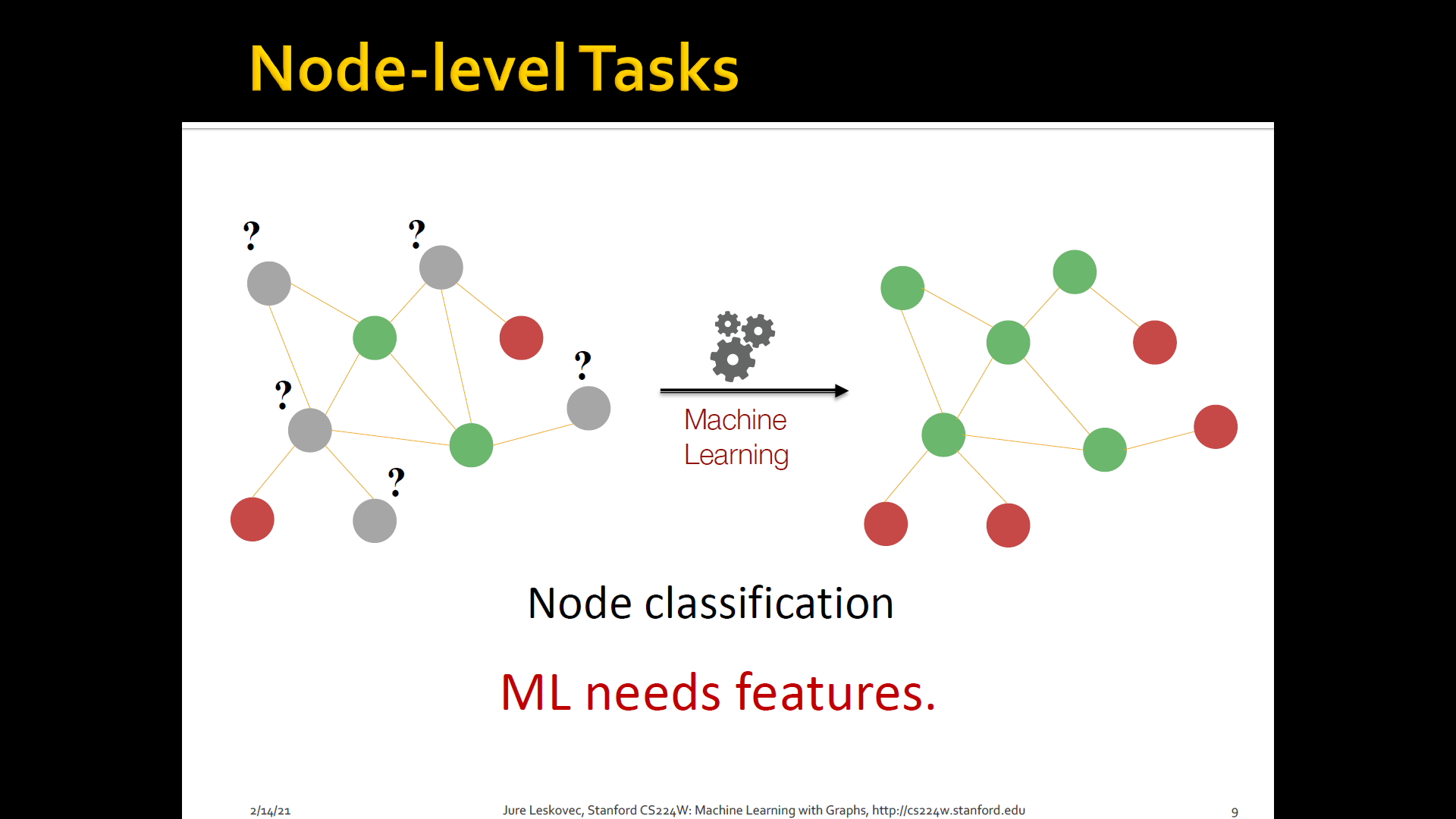
- Using effective features over graphs is the key to achieving good test performance
-
ML in Graphs
-
Given
-
Learn a function
-
The way we can think of this is that we are given a graph as a set of verticies, as a set of edges and we wanna learn a function
-
2.1 Node-level tasks and features
-
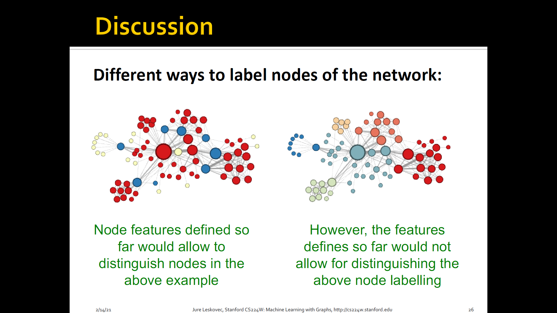
Node classification: Where we are given a network, we are given a couple of nodes that are labeld with different colors, and the goal is to predict the colors of uncolored nodes
-
Goal: Characterize the structure and position of a node in the network
- Node degree
- Node centrality
- Clustering coefficient
- Graphlets
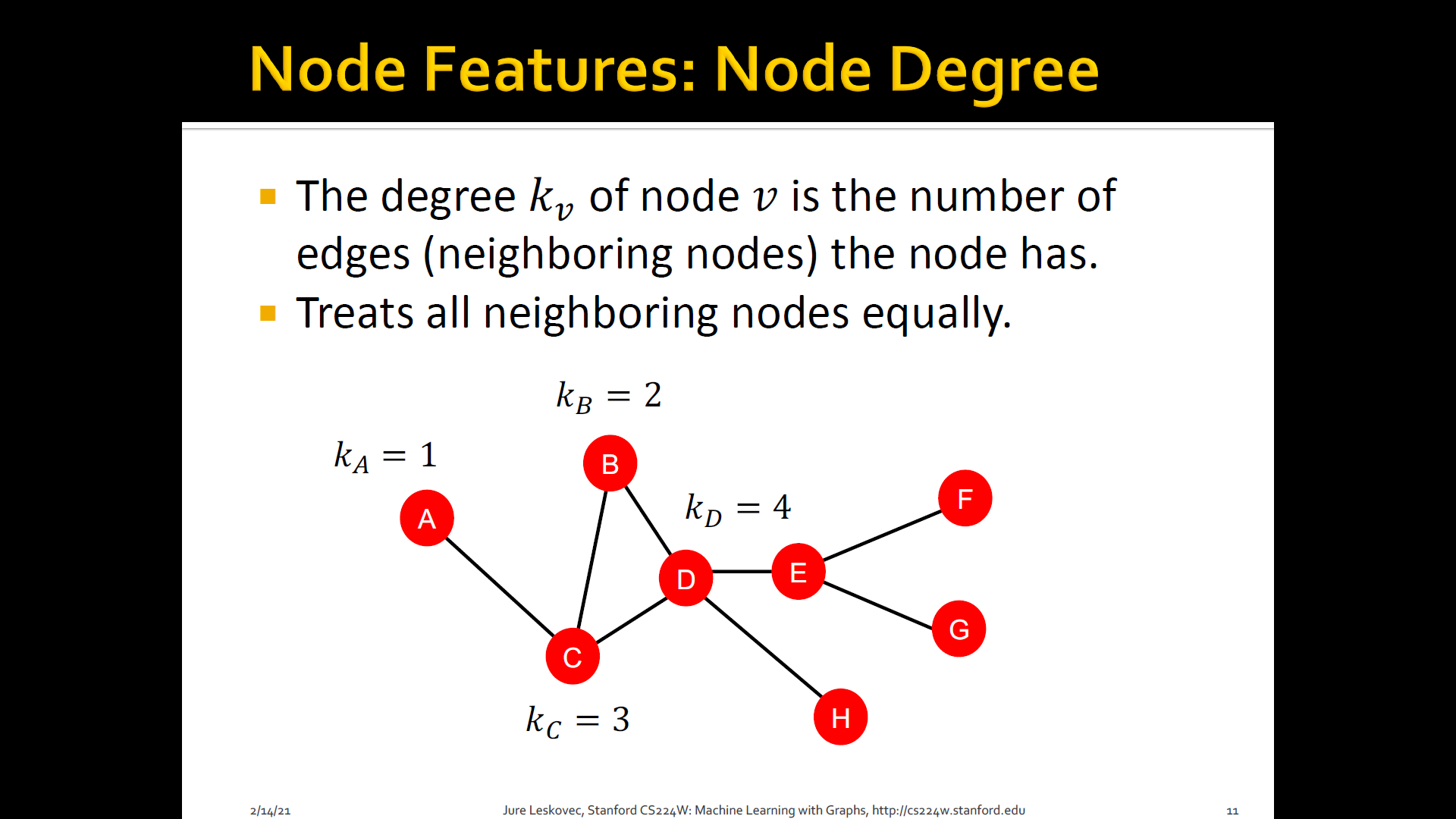
1. Node degree
- The degree of of is the number of edges (neighboring nodes) the node has
- Treats all neighboring nodes equally
2. Node centrality
-
Node degree counts the neighboring nodes without capturing their importance
-
Node centrality takes the node importance in a graph into account
-
Different ways to model importance
- Eigen-vector centrality
- Betweenness centrality
- Closeness centrality
- and many others
-
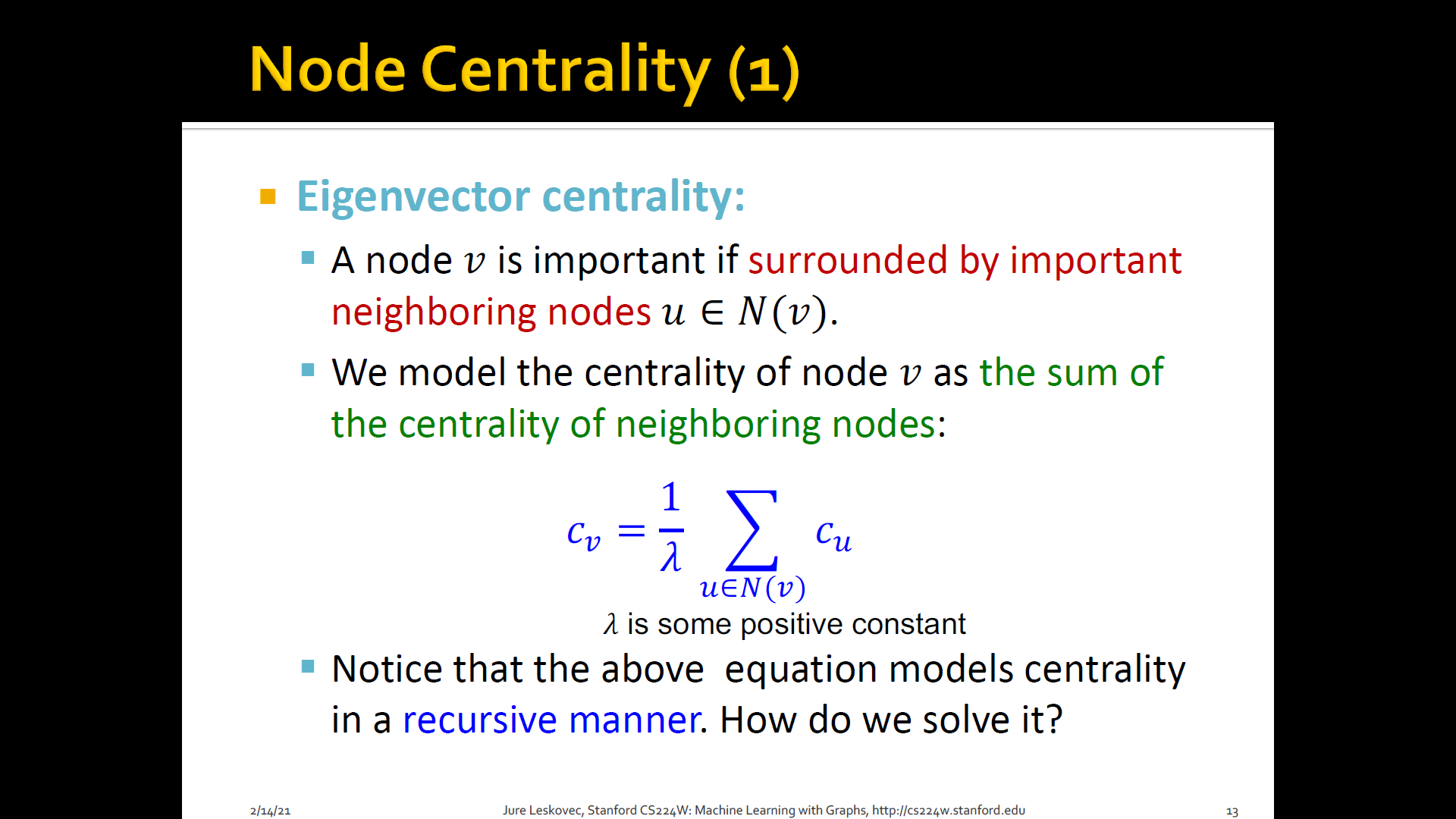
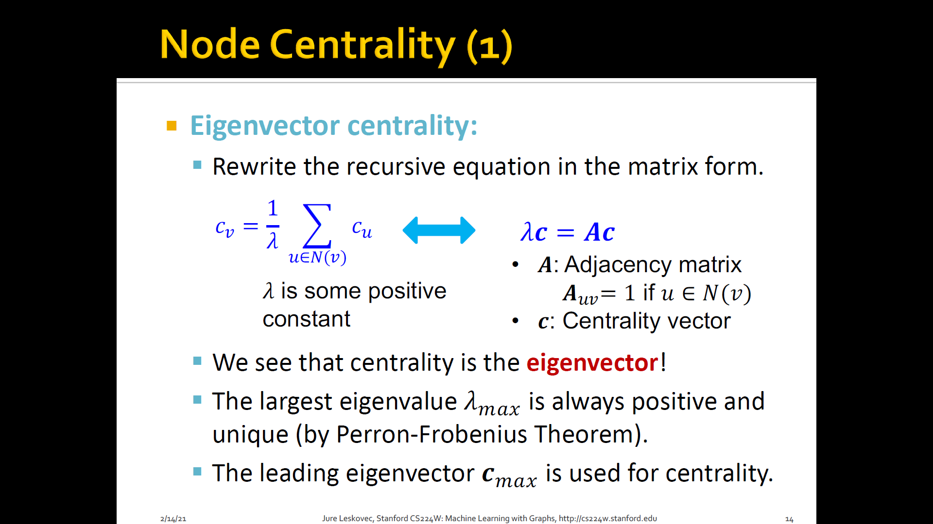
Eigen-vector centrality: A node is important if surrounded by important neighboring nodes
-
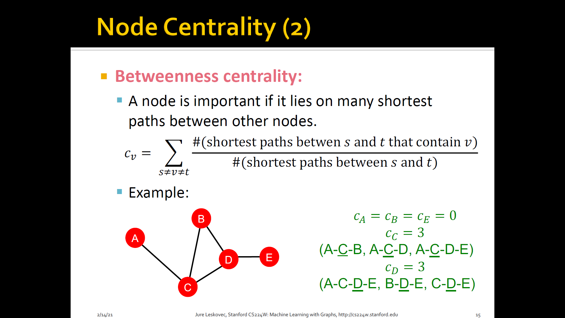
Betweenness centrality: A node is important if it lies on many shortest paths b/t other nodes
-
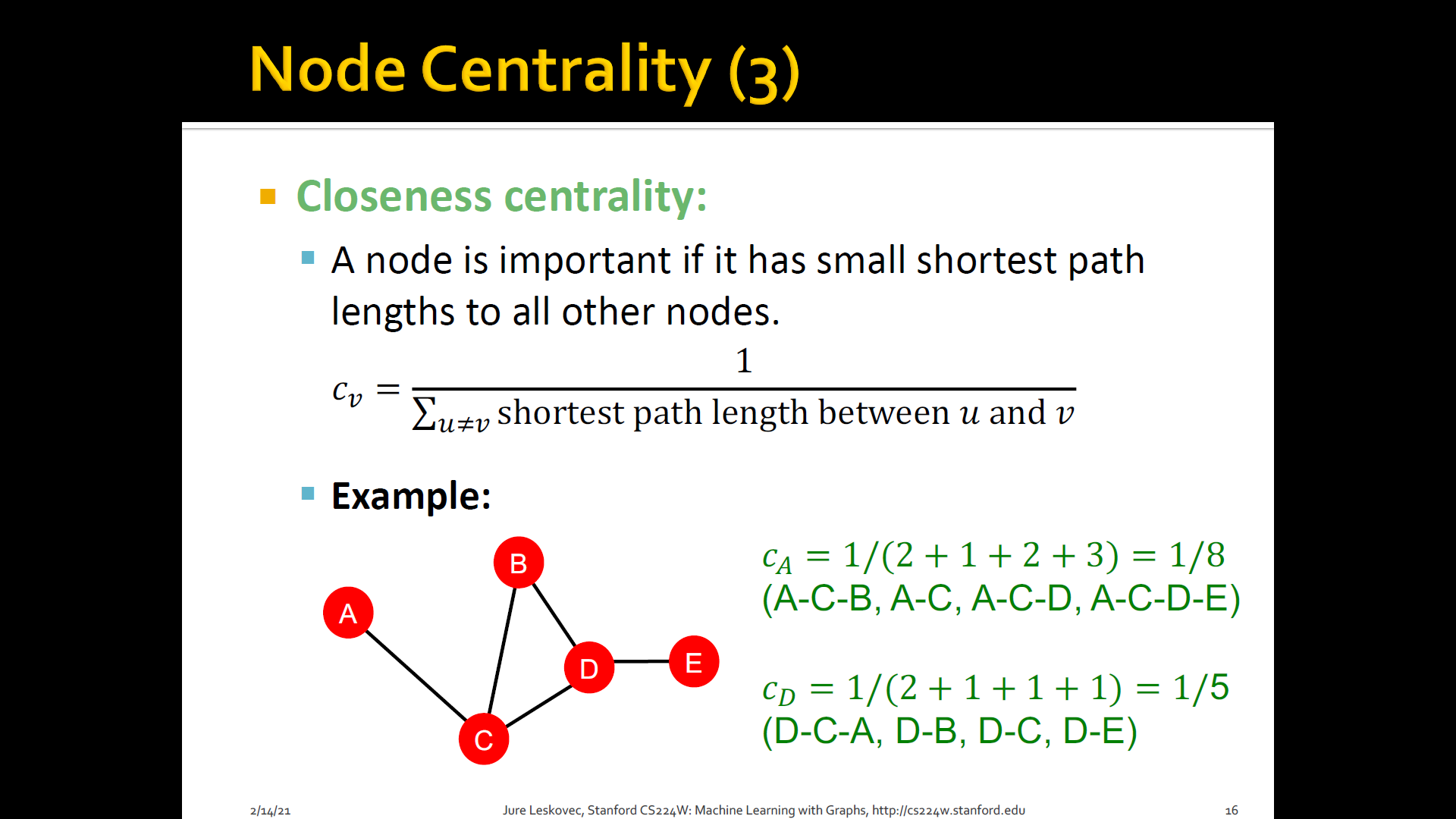
Closeness centrality: A node is important if it has small shortest path lengths to all other nodes
3. Clustering coefficient
- Measures how connected neighboring nodes

4. Graphlets
-
Observation: Clustering coeffieicnt counts the #(triangles) in the ego-network
-
We can generalize the by #(pre-specified subgraphs, i.e. graphlets)

-
Graphlets: Rooted connected non-isomorphic subgraphs

-
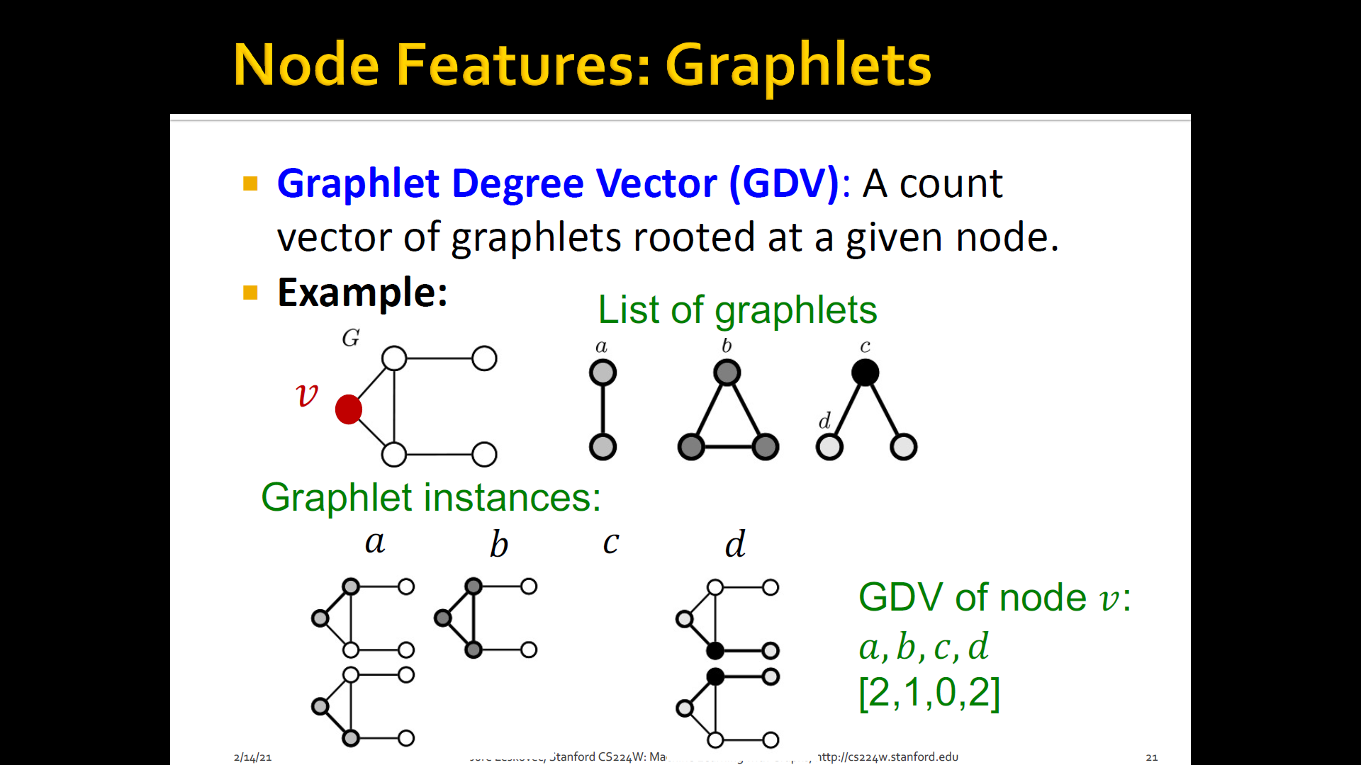
GDV(Graphlet Degree Vector): Graphlet-base features for nodes
- Degree counts #(edges) that a node touches
- Clustering coefficient counts #(triangles) that a node touches
- GDV counts #(graphlets) that a node touches
-
GDV(Graphlet Degree Vector): A count vector of graphlets rooted at a given node
-
Considering graphlets on 2 to 5 nodes we get:
- Vector of 73 coordinates is a signature of a node that describes the topology of node's neighborhood
- Captures its inter-connectivities out to a distance of 4 hops
-
Graphlet degree vector provides a measure of a node's local network topology:
- Comparing vectors of two nodes provides a more detailed measure of local topological similarity than node degrees or clustering coefficient
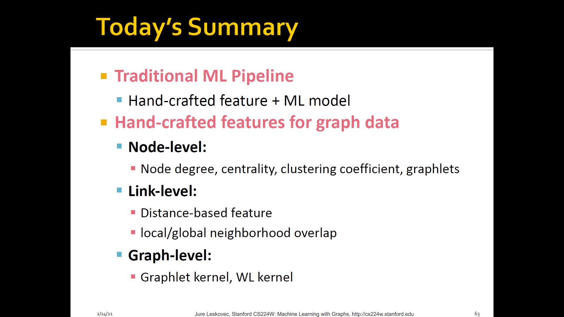
Summary
2.2 Link prediction task and features
-
The link prediction task is to predict new links based on existing links
-
At test time, all node pairs(no existing links) are ranked, and top node pairs are predicted
-
The key is to design features for a pair of nodes
-
Two formulations of the link prediction task
- Links missing at random
- Remove a random set of links and then aim to predict them
- More useful for static networks like protein-protein interaction networks
- Links over time
- Given a graph on edges up to time , output a ranked list of links (not in ) that are predicted to appear in
- Evaluation
- : # new edges that appear during the test period
- Take top elements of and count correct edges
- Useful or natural for networks that evolve over time like transaction networks, social networks
- Links missing at random
-
Methodology
- For each pair of nodes compute score
- For example, could be the # of common neighbors of and
- Sort pairs by the decreasing score
- Predict top pairs as new links
- See which of these links actually appear in
-
Link-level features:
- How to featurize or create a descriptor of the relationship b/t two nodes in the network
- Distance-based feature
- Local neighborhood overlap
- Global neighborhood overlap
1. Distance-based features
- Shortest path distance b/t two nodes
- However, this does not capture the degree of neighborhood overlap(=strength of connection)

2. Local neighborhood overlap
- Try to capture the strength of connection b/t two nodes would be to ask how many neighbors do you have in common
- What is the number of common friends b/t a pair of nodes
- Captures # neighboring nodes shared b/t two nodes and
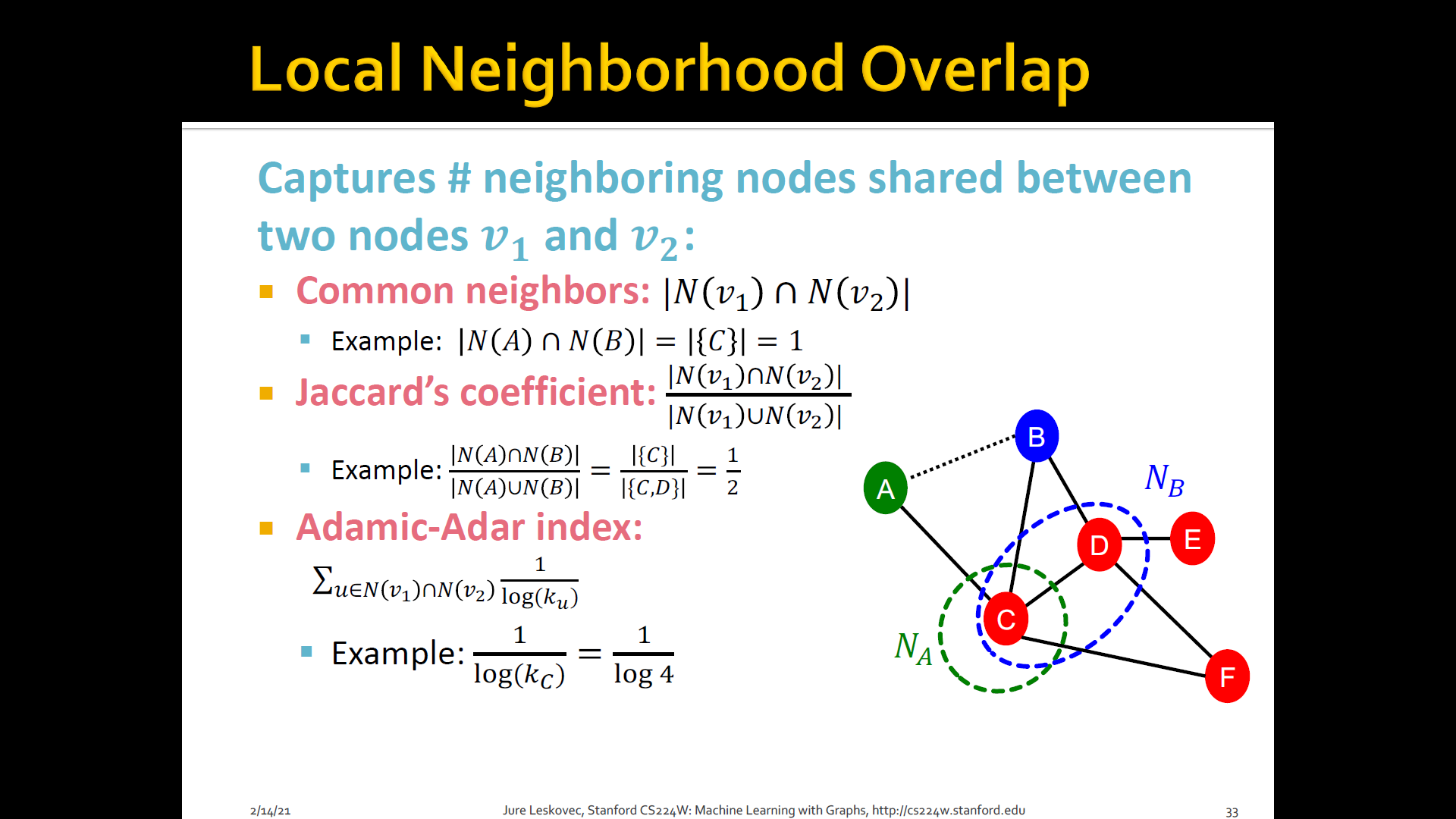
- Limitation: Is always zero if the two nodes do not have any neighbors in common (However, the two nodes may still potentially be connected in the future)
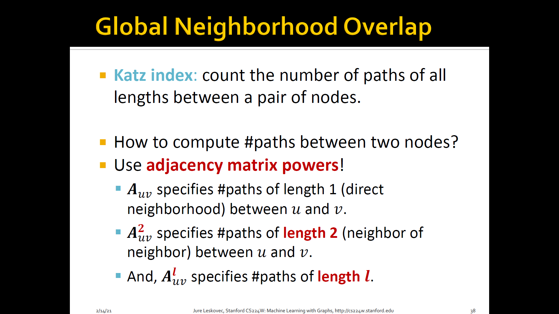
3. Global neighborhood overlap
- Resolve the limitation of local neighborhood overlap by considering the entire graph
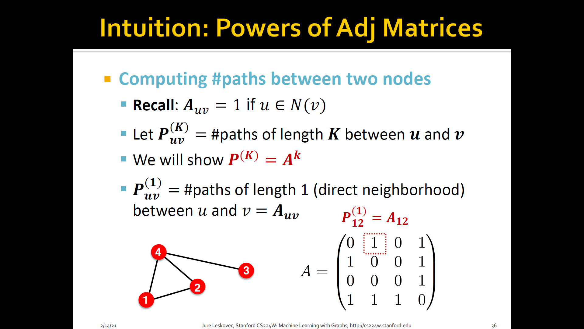
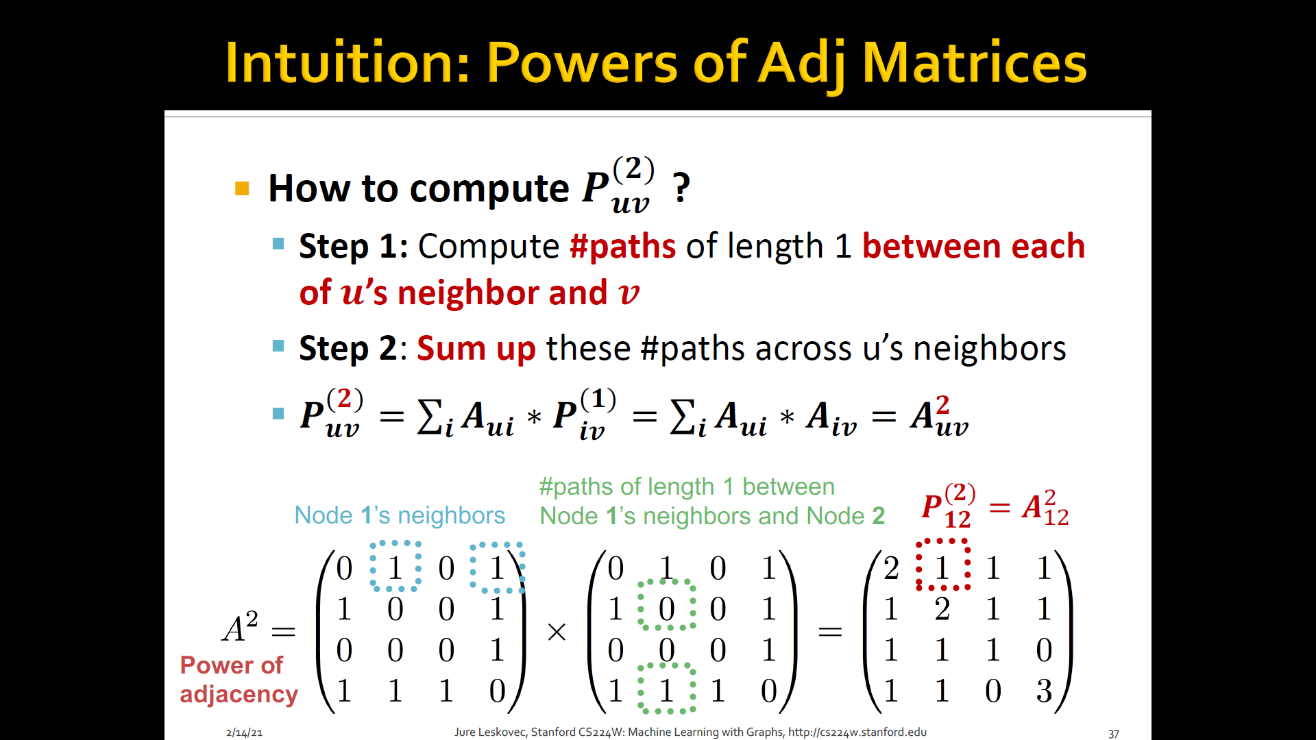
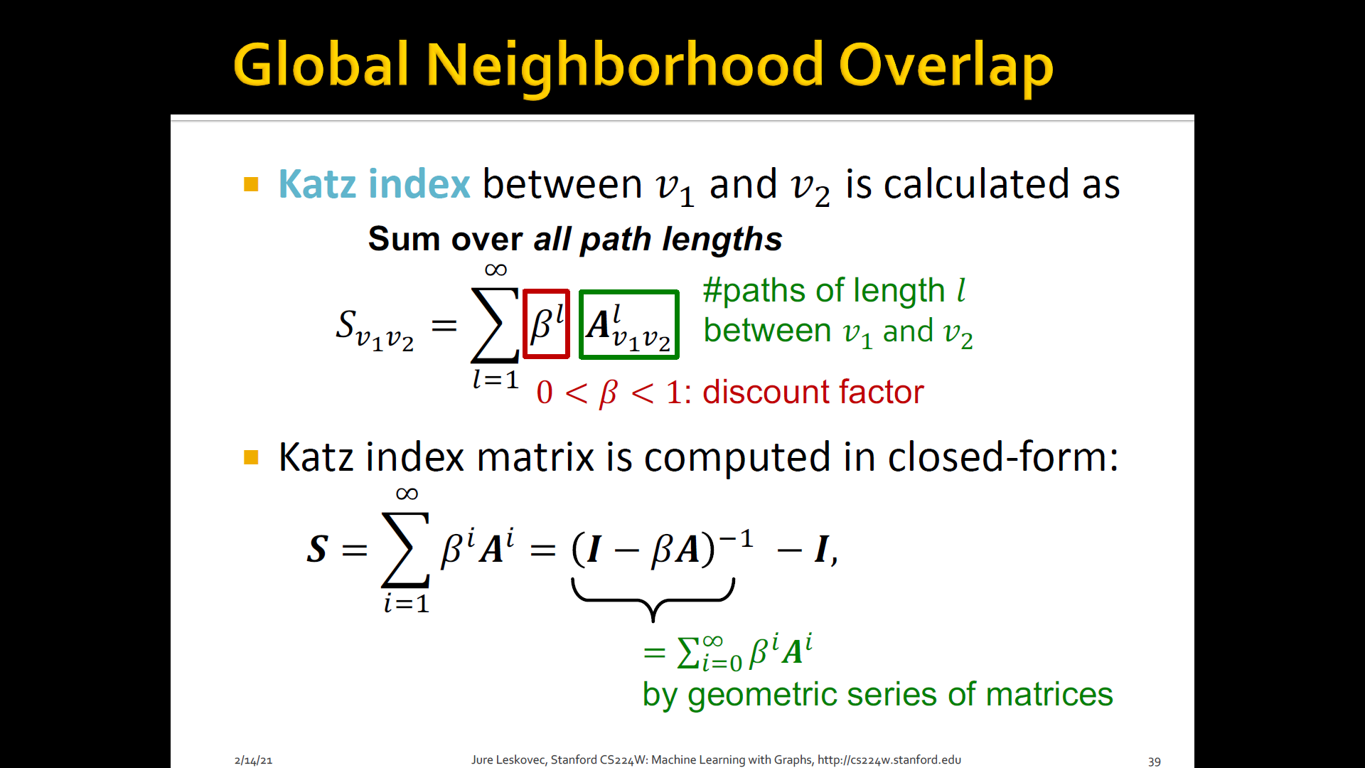
- Katz index: count the number of paths of all lengths b/t a given pair of nodes
- How to compute # paths b/t two nodes?
- Use adjacency matrix
Summary

2.3 Graph-level features and Graph kernels
-
Features that characterize the structure of an entire graph
-
Kernel methods are widely-used for traditional ML for graph-level prediction
- IDEA: Design kernels instead of feature vectors
- A quick introduction to Kernels
- Kernel measures similarity b/t data
- Kernel matrix must always be positive semi-definite (i.e., has positive eigenvalues)
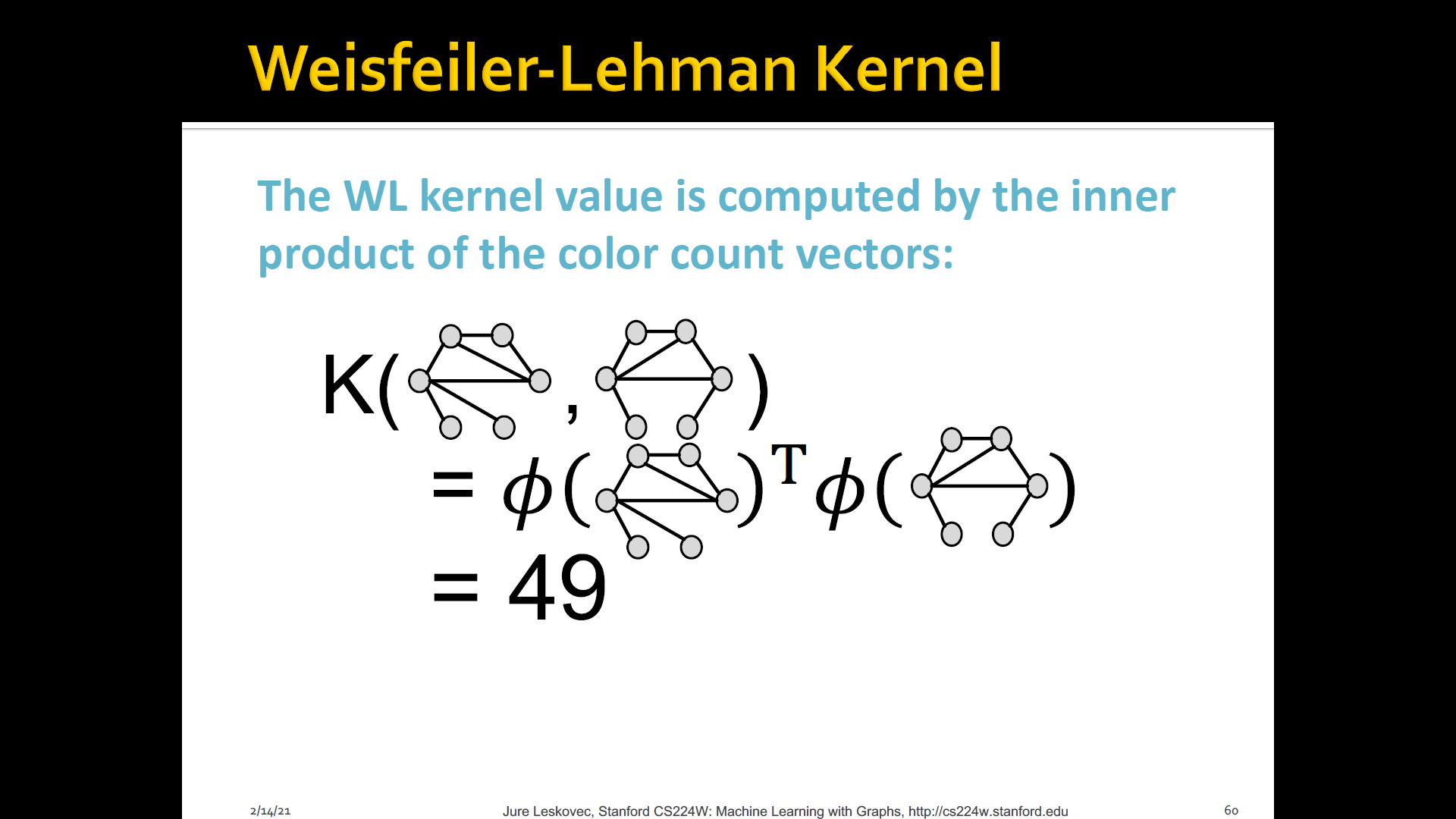
- There exists a feature representation such that
- And the value of the kernel is simply a dot product of this vector representation of the two graphs
- Once the kernel is defined, off-the-shelf ML model, such as kernel SVM can be used to make predictions
-
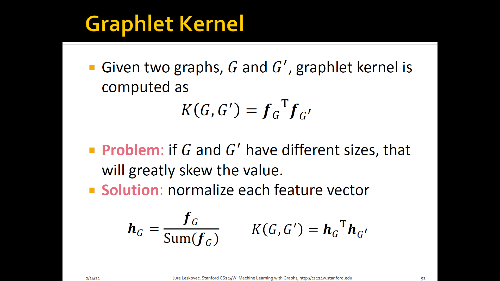
Graph Kernels: Measure similarity b/t two graphs
- Goal: Design graph feature vector
- Key IDEA: BoW(Bag-of-Words) for a graph
- BoW simply uses the word counts as features for documents (no ordering considered)
[1] Graphlet kernel
[2] WL(Weisfeiler-Lehman) kernel
[3] Other kernels are also proposed in the literature- Random-walk kernel
- Shortest-path graph kernel
- And many more
-
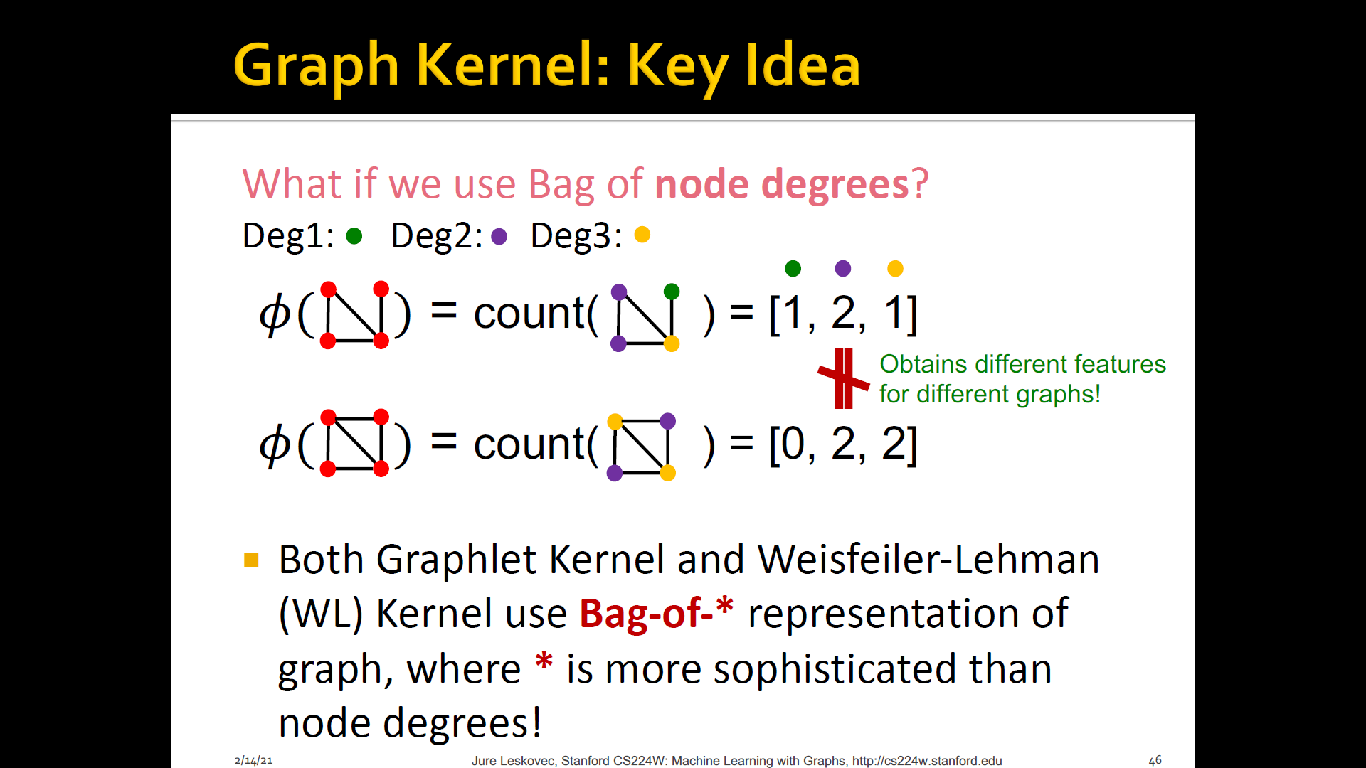
Both Graphlet kernel and WL kernel use Bag-of-* representation of graph, where * is more sophisticated than node degress
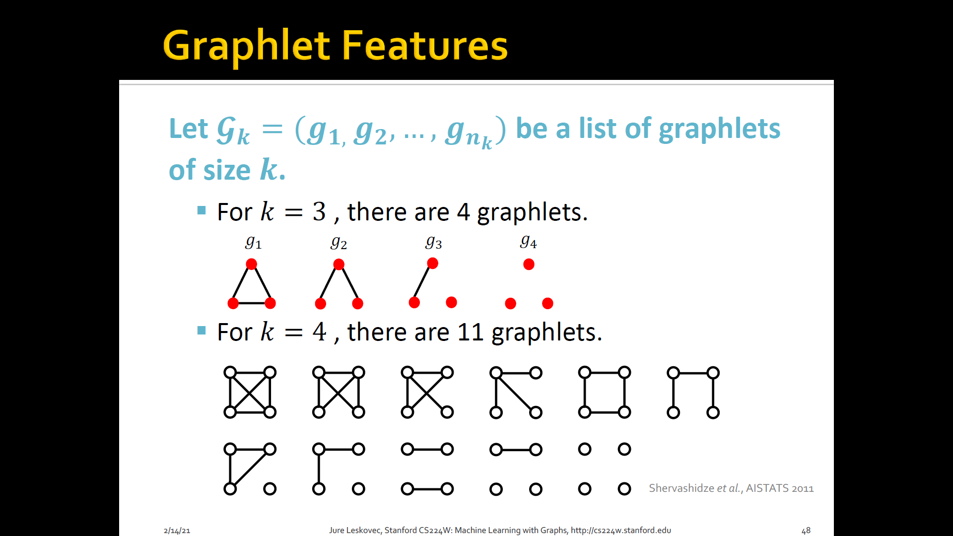
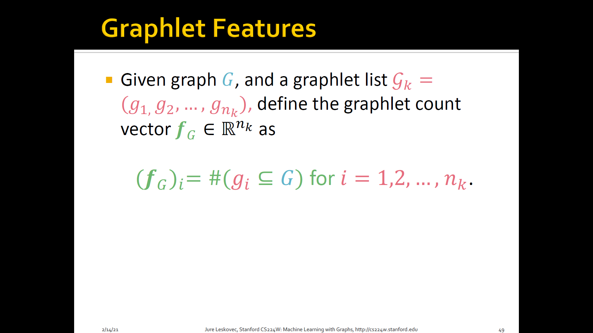
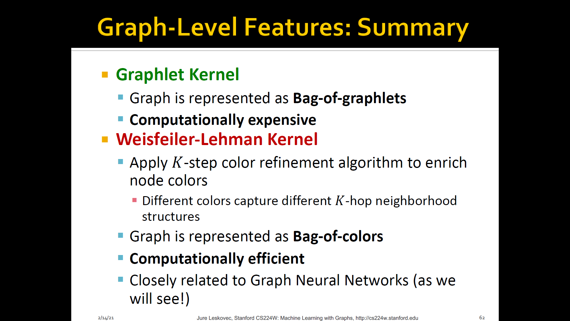
1. Graphlet features
-
Count the number of different graphlets in a graph
-
Definition of graphlets here is slightly different from node-level features
-
Two two differences are
- Nodes in graphlets here do not need to be connected (allows for isolated nodes)
- The graphlets here are not rooted

-
Limitations: Counting graphlet is expensive
-
Counting size- graphlets for a graph with size by enumeration takes
-
This is unavoidable in the worst-case since subgraph isomorphism test (judding whether a graph is a subgraph of another graph) is NP-hard
-
If a graph's node degree is bounded by , an algorithm exists to count all the graphlets of size
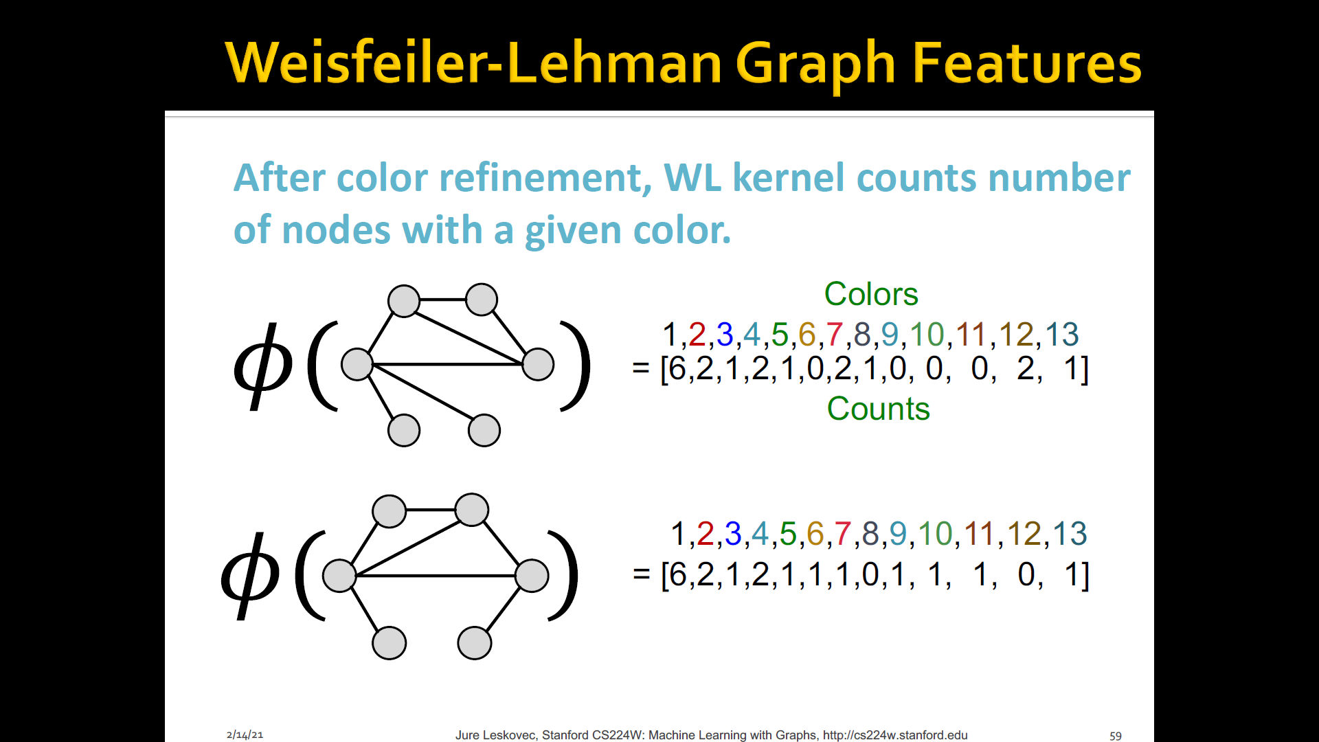
2. WL(Weisfeiler-Lehman) Kernel
-
Goal: Design an efficient graph feature descriptor of
-
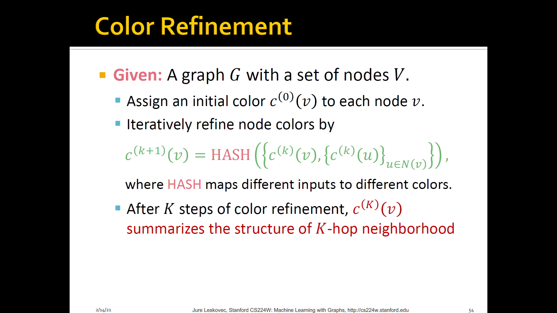
IDEA: Use neighborhood structure to iteratively enrich node vocabulary
- Generalized version of Bag-of-node degrees since node degrees are one-hop neighborhood information
- Algorithm to achieve this: WL graph isomorphsim test(=Color refinement)
-
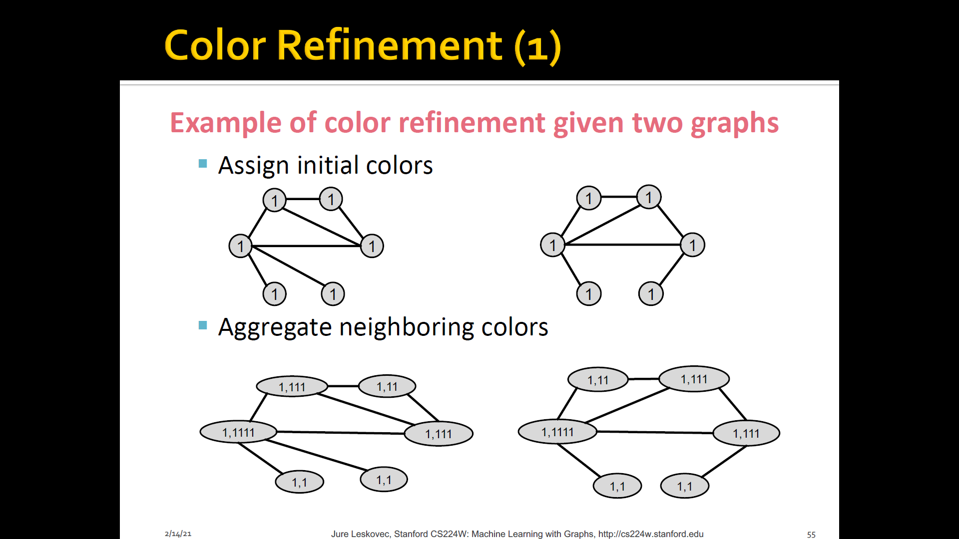
Color refienment

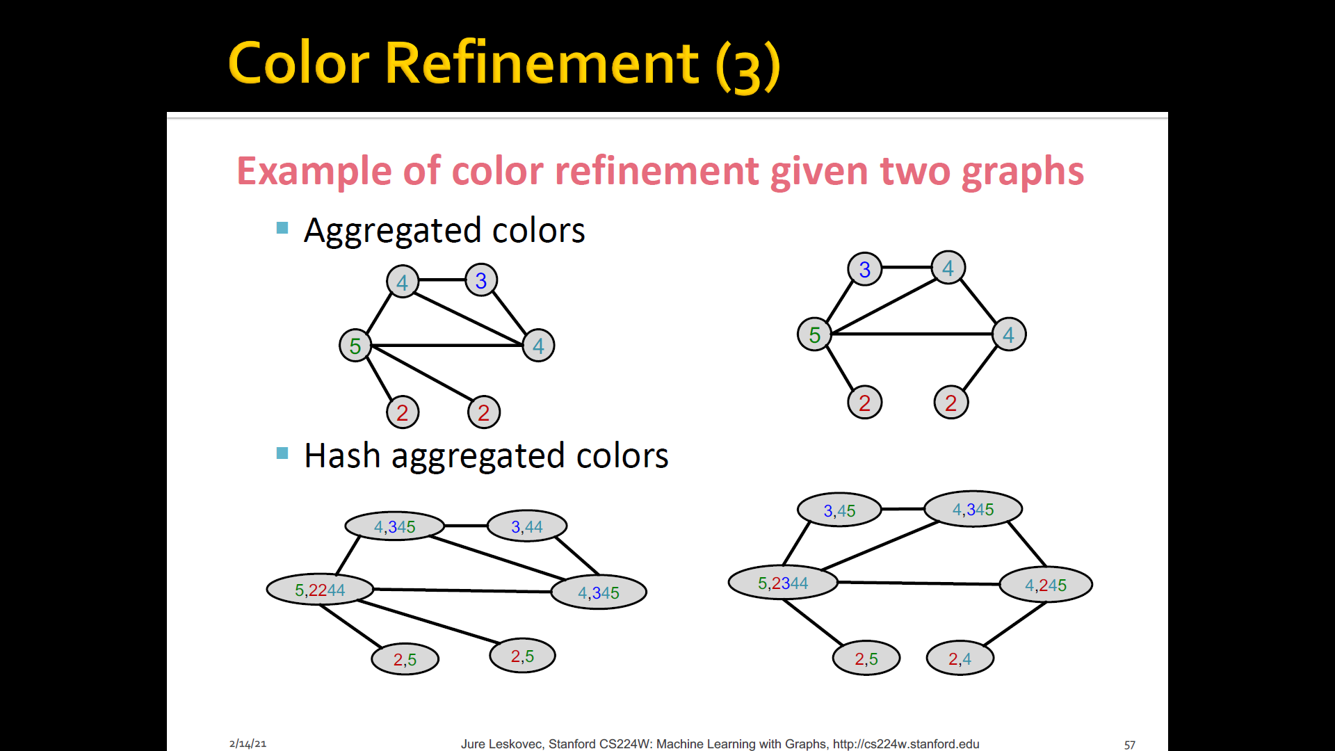
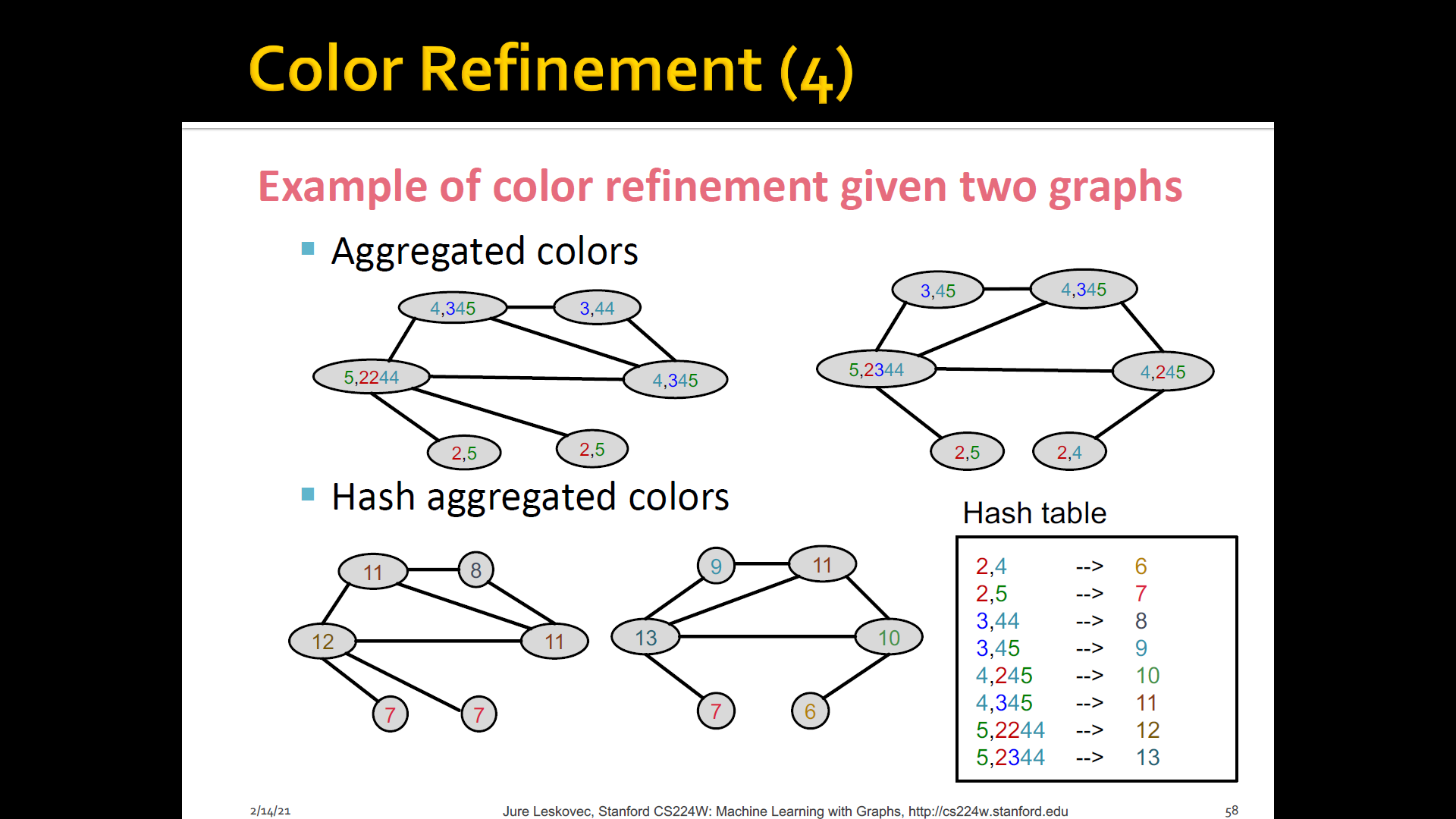
-
WL kernel is very popular/strong graph feature descriptor to gives strong performance and computationally efficient
- The time complexity for color refinement at each step is linear in #(edges), since it involves aggregating neighboring colors
- When computing a kernel value, only colors appeared in the two graphs need to be tracked
- Thus, #(colors) is at most the total number of nodes
- Counting colors takes linear-time w.r.t #(nodes)
- In total, time complexity is linear in #(edges)
Sumamry
Lecture Summary