Graph Representation Learning

3.1 Node Embeddings

• Recap: Traditional ML for graphs

  • Given an input graph, extract node, link and graph-level features, learn a model that maps features to labels
  • Input graph → Structured features → Learning algorithm → Prediction

• Graph tepresentation learning

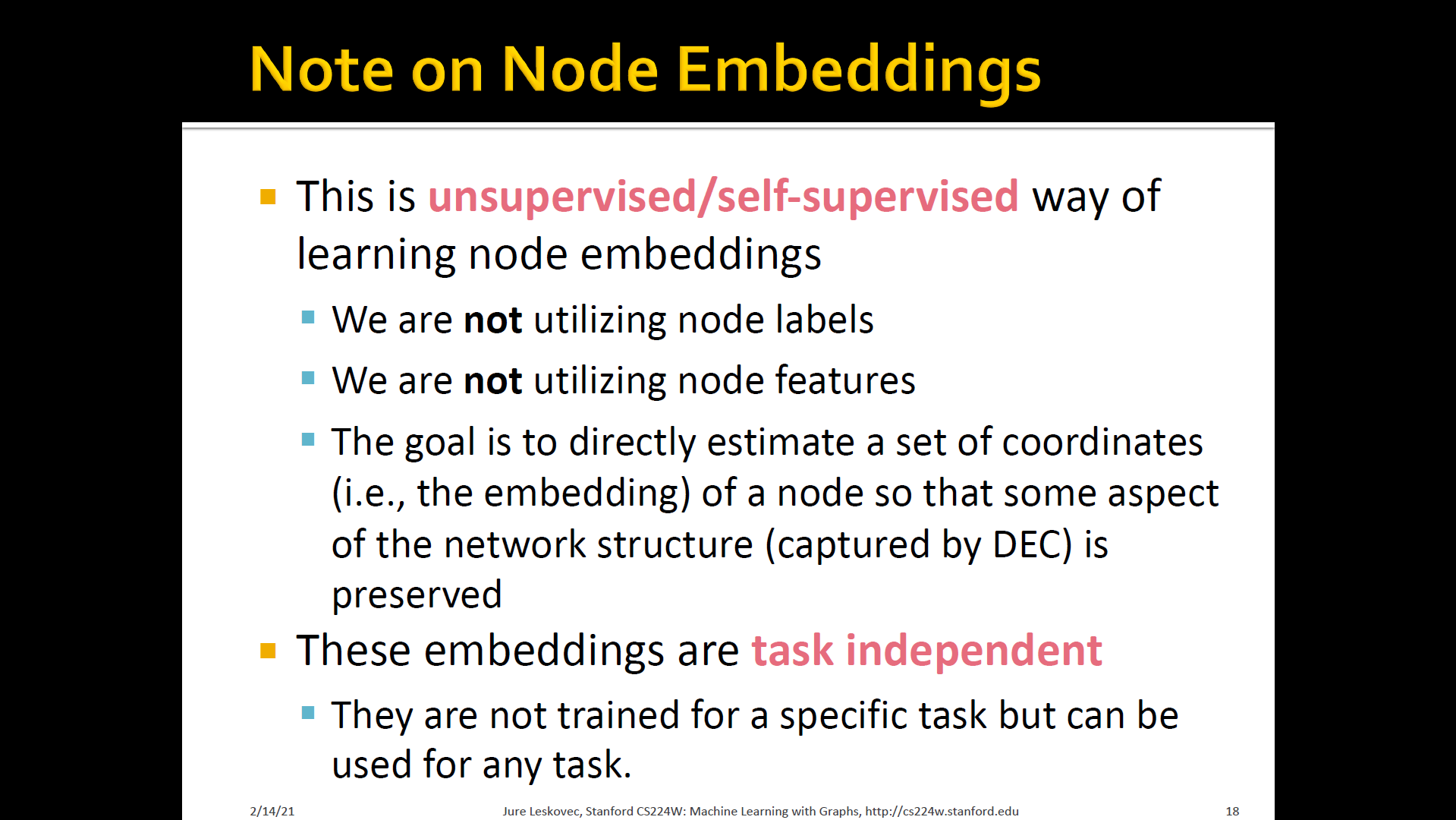
  • Graph representation learning alleviates the need to do feature engineering every single time → Automatically learn the features
  • Learn how to map node in a d-dimensional space and represent it as a vector of d numbers
  • Call it this vector of d numbers as feature representation or embedding
    • This vector captures the structure of the underlying network that we are interested in analyzing or making predictions over

• Why embedding?

  • Task: Map node into an embedding space
  • Similarity of embeddings b/t nodes indicates their similarity in the network
    • For example: Both nodes are close to each other (connected by an edge)
  • Encode network structure information
  • Potentially used for many downstream predictions
    • Node classification, Link prediction, Graph classification, Anomalus node detection, Clustering and so on

Encoder and Decoder

• Assume we have a graph $G$:
  • $V$ is the vertex set
  • $A$ is the adjacency matrix (assume binary)
  • For simplicity: no node features or extra information is used

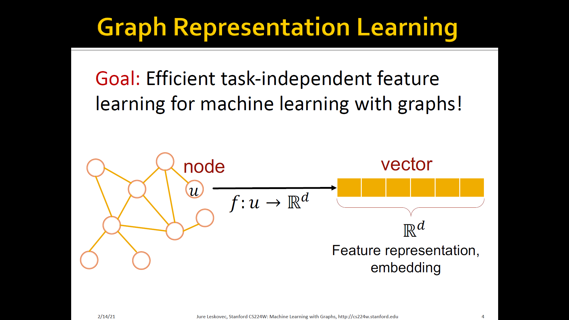
• Embedding nodes

  • Encode nodes so that similarity in the embedding space (e.g, dot-product) approximates similarity in the graph
  • To learn encoder that encodes the original networks as a set of node embeddings
    

• Learning node embeddings

  1. Encoder maps from nodes to embeddings
  2. Define a node similarity function (i.e, a measure of similarity in the original network)
  3. Decode maps from embeddings to the similairty score
  4. Optimize the parameters of the encoder

• Two key components

  • Encoder: maps each node to a low-dimensional vector
  • Similarity function: specifies how the relationships in vector space map to the relationships in the original network

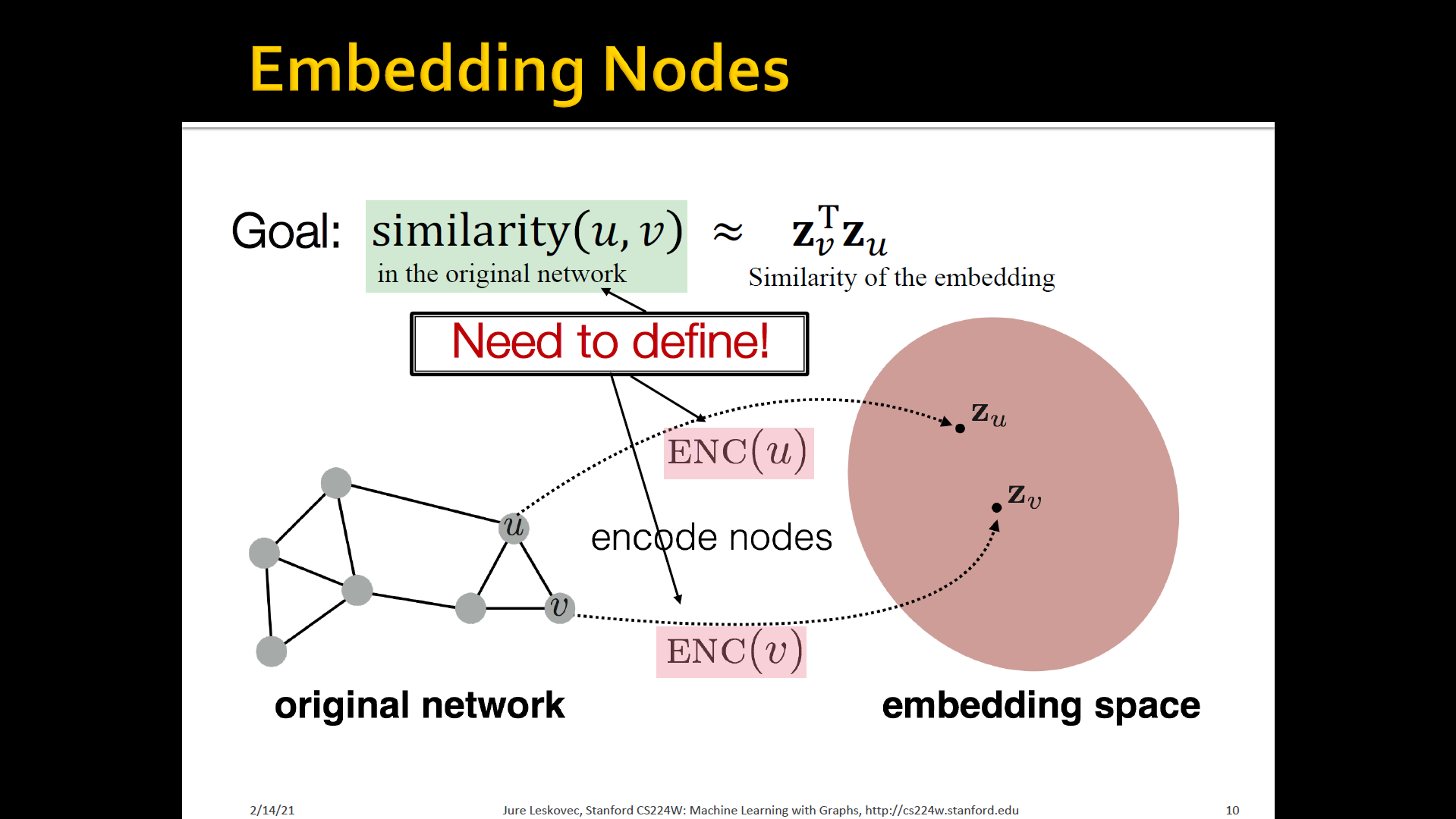
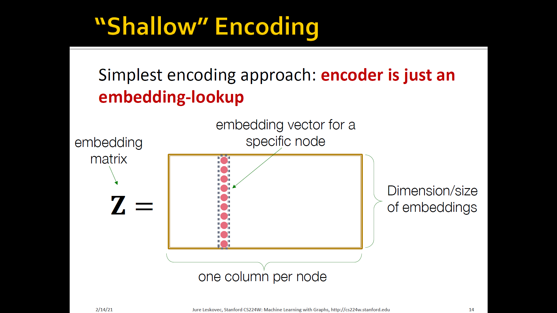
• Shallow eEncoding

  • Simplest encoding approach: Encoder is just an embedding-lookup
  • Each node is assigned a unique embedding vector (i.e, we directly optimize the embedding of each node): DeepWalk, Node2Vec
    

• Encoder + Decoder framework

  • Shallow encoder: embedding lookup
  • Parameters to optimize: $Z$ which contains node embeddings $z_u$ for al nodes $u \in V$
  • Decoder: based on node similarity
  • Objective: maximize ${z_v}^Tz_u$ for node pairs $(u, v)$ that are similar according to our node similairty function

• How to define node similarity?

  • Should two nodes have a similar embedding if they
    • are linked?
    • share neighbors?
    • have similar "structural roles"?
  • Similarity definition that uses random walks, and how to optimize embeddings for such a similarity measure

Summary

3.2 Random walk approaches for node embddings

• Notation
  • Vector $z_u$: The embedding of node $u$ (what we aim to find)
  • Probability $P(v|z_u)$: The (predicted) probability of visiting node $v$ on random walks starting from node $u$. (Our model prediction based on $z_u$
• Non-linear functions used to produce predicted probabilities $P(v|z_u)$
  • Softmax function: Turns vector of $K$ real values (model predictions) into $K$ probabilities that sum to 1
  • Sigmoid function: S-shaped function that turns real values into the range of (0, 1)

• Random walk
  • Given a graph and a starting point(node), we select a neighbor of it at random, and move to this neighbor
  • Then we select a neighbor of this point at random, and move to it
  • The (random) sequence of points visited this way is random walk on the graph

• Random walk embeddings: ${z_u}^Tz_v \approx$ probability that $u$ and $v$ co-occur on a random walk over the graph
  1. Estimate probability of visiting node $v$ on a random walk starting from node $u$ using some random walk strategy $R$
  2. Optimize embeddings to encode these random walk statistics
     • Similarity in embdding space(Here: dot product = $cos(\theta)$) encodes random walk "similarity"
• Why random walks?
  • Expressitivity: Flexible stochastic definition of node similarity that incorporates both local and higher-order neighborhood information
    • IDEA: if random walk starting from node $u$ visits $v$ with high probability, $u$ and $v$ are similar (high-order multi-hop information)
  • Efficiency: Do not need to consider all node pairs when training; only need to consider pairs that co-occur on random walks
• Un-supervised feature learning
  • Intuition: Find embedding of nodes in $d$-dimensional space that preserves similarity
  • IDEA: Learn node embedding such that near by nodes are close together in the network
  • Given a node $u$, how do we define neraby nodes?
    • $N_R(u)$ ... neighborhood of $u$ obtained by some random walk strategy $R$
• Feature learning as Optimization
  • Given $G=(V, E)$
  • Our goal is to learn a mapping $f: u-> \R^d:f(u)=z_u$
  • Log-likelihood objective $\max_{f} \displaystyle\sum_{u\in V}logP(N_R(u)|z_u)$
    • $N_R(u)$ is the neighborhood of node $u$ by strategy $R$
• Given node $u$, we want to learn feature representations that are predictive of the nodes in its random walk neighborhood $N_R(u)$

• Random walk optimization

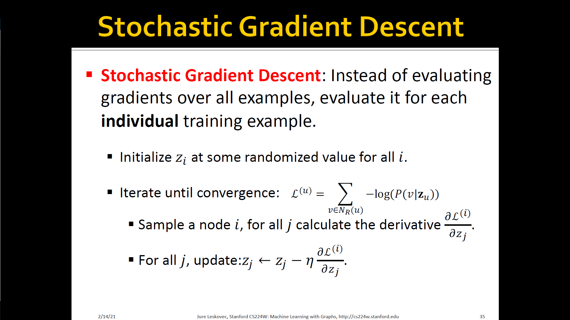
  1. Run short-fixed length random walks starting from each node $u$ in the graph using some random walk strategy $R$
  2. For each node $u$ collect $N_R(u)$, the multiset of nodes visited on random walks starting from $u$
     • $N_R(u)$ can have repeat elements since nodes can be visited multiple times on random walks
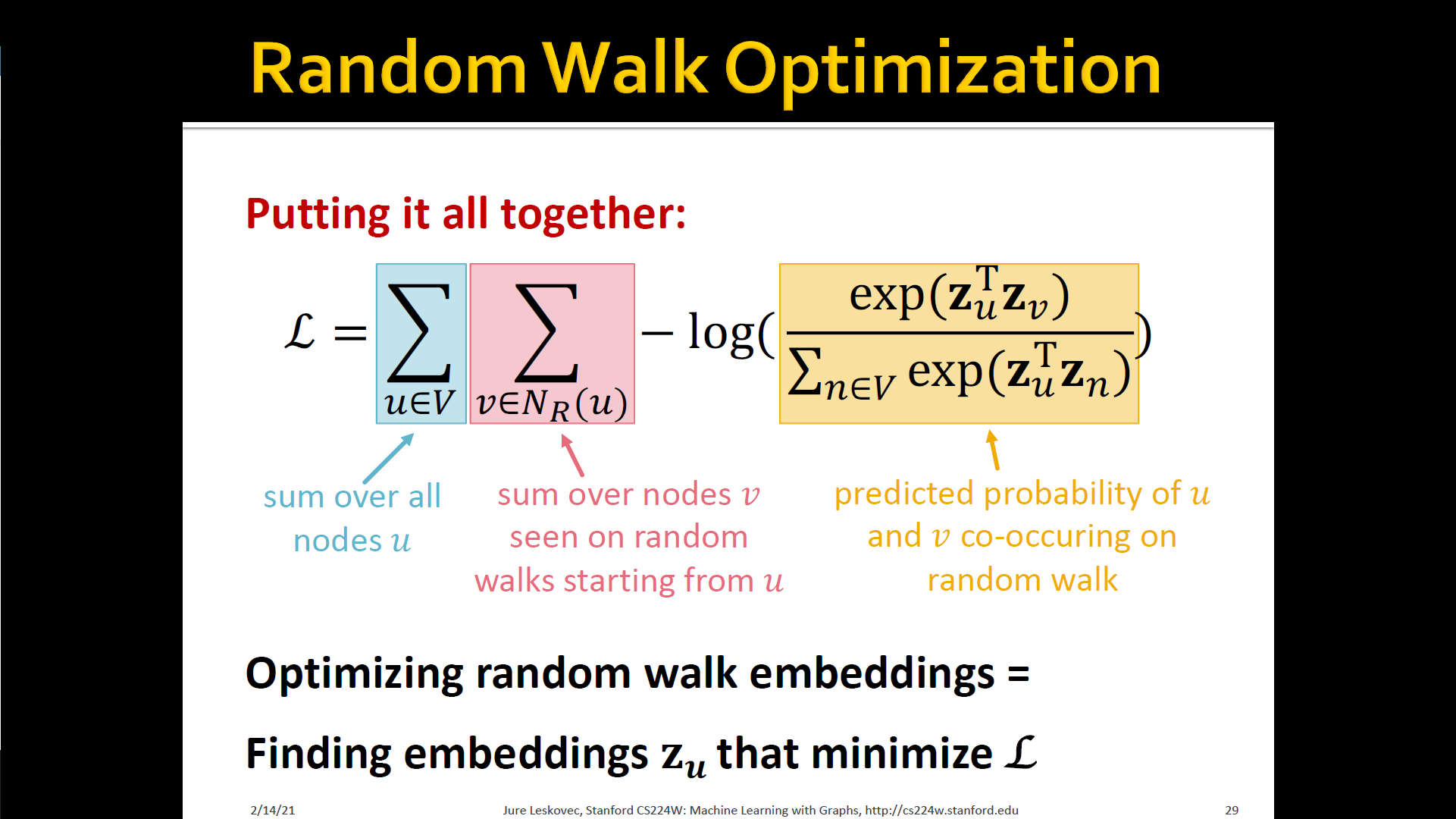
  3. Optimize embeddings according to: Given node $u$, predicts its neighbors $N_R(u)$
     • $\max_{f} \displaystyle\sum_{u\in V}logP(N_R(u)|z_u)$ → maximum likelihood objective
  4. Equivalently,
     $L = \displaystyle\sum_{u \in V}\sum_{v \in N_R(u)}-log(P(v|z_u))$
     • Intuition: Optimize embeddings $z_u$ to maximize the likelihood of random walk co-occurrences
     • Parameterize $P(v|z_u)$ using softmax:
       $P(v|z_u) = {exp({z_u}^Tz_v) \over \sum_{n \in V} exp({z_u}^Tz_n)}$
       

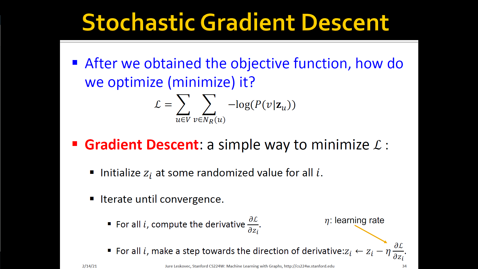
• Stochastic Gradient Descent

  • 

Random walks summary

Node2Vec

• How sould we randomly walk?
  • So far, we have described how to optimize embeddings given a random walk strategy $R$
  • What strategies should we use to run these random walks?
    • Simplest idea: Just run fixed-length, unbiased random walks strating from each node (DeepWalk)
      • The issue is that such notion of similarity is too constrained
• Overview of Node2Vec
  • Goal: Embed nodes with similar network neighborhoods close in the feature space
  • We frame this goal as a maximum likelihood optimization problem, independent to the downstream prediction task
  • Key observation: Flexible notion of network neighborhood $N_R(u)$ of node $u$ leads to rich node embeddings
  • Develop biased $2nd$ order random walk $R$ to generate network neighborhood $N_R(u)$ of node $u$
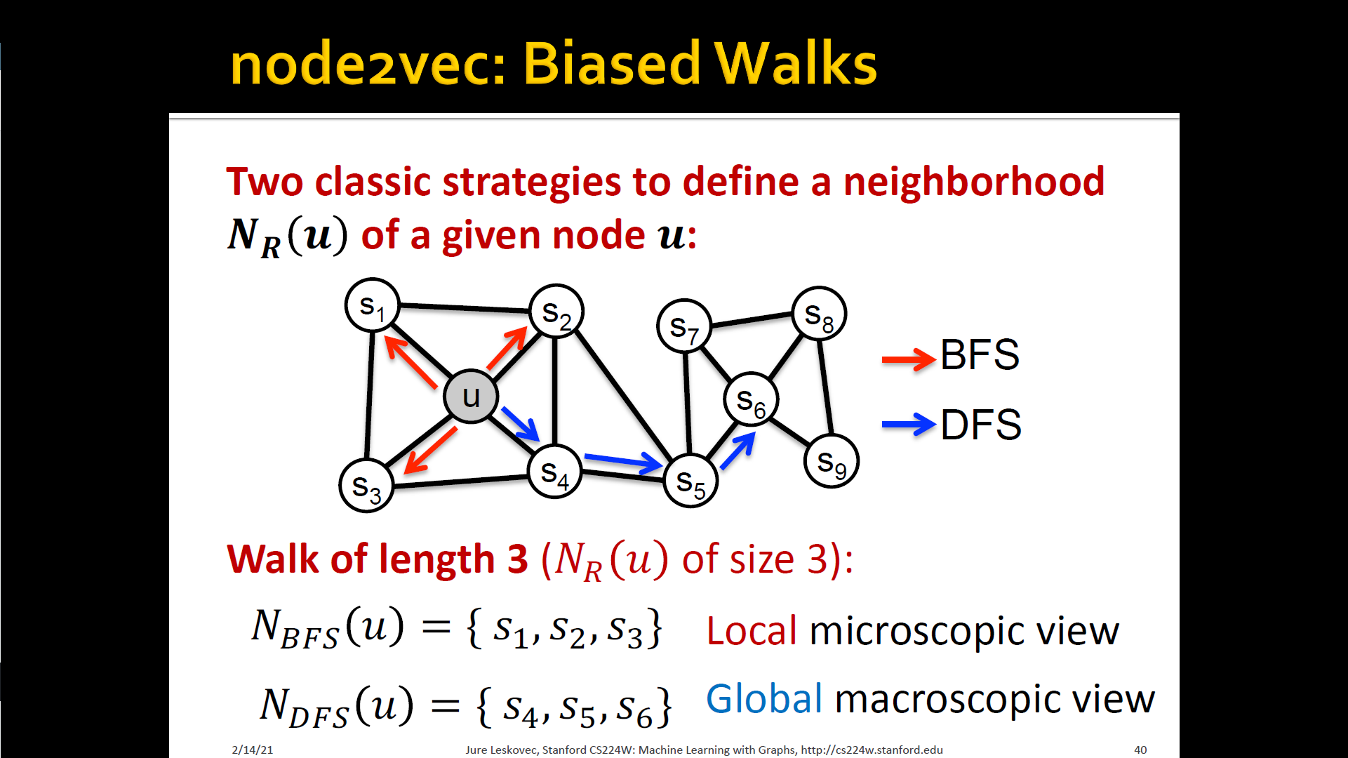
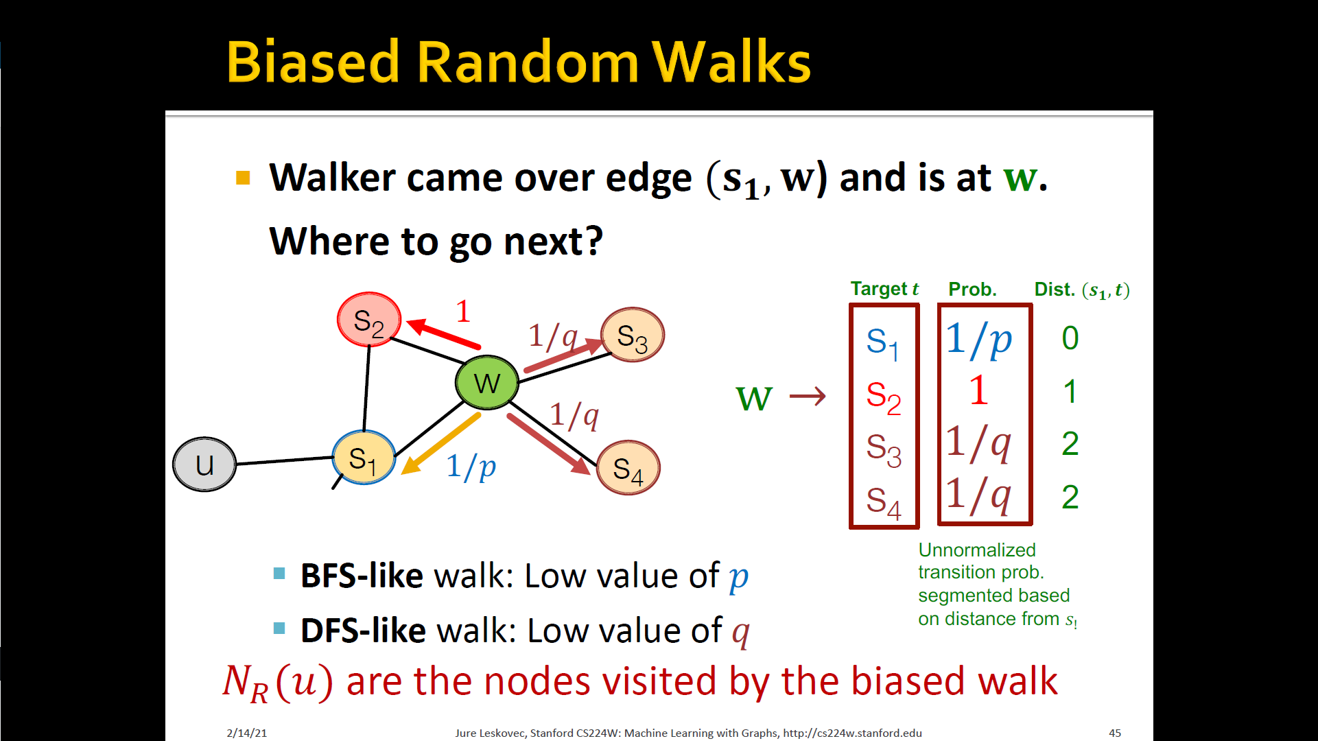
• Node2Vec : Biased walks
  • IDEA: use flexible, biased random walks that can trade-off b/t local and global vies of the network

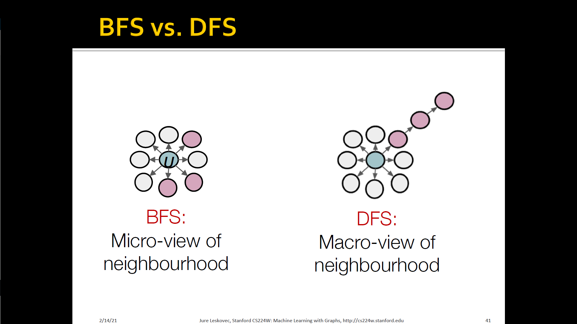
• Interpolating BFS and DFS

  • Biased fixed-length random walk $R$ that given a node $u$ generates neighborhood $N_R(u)$
    • Two parameters
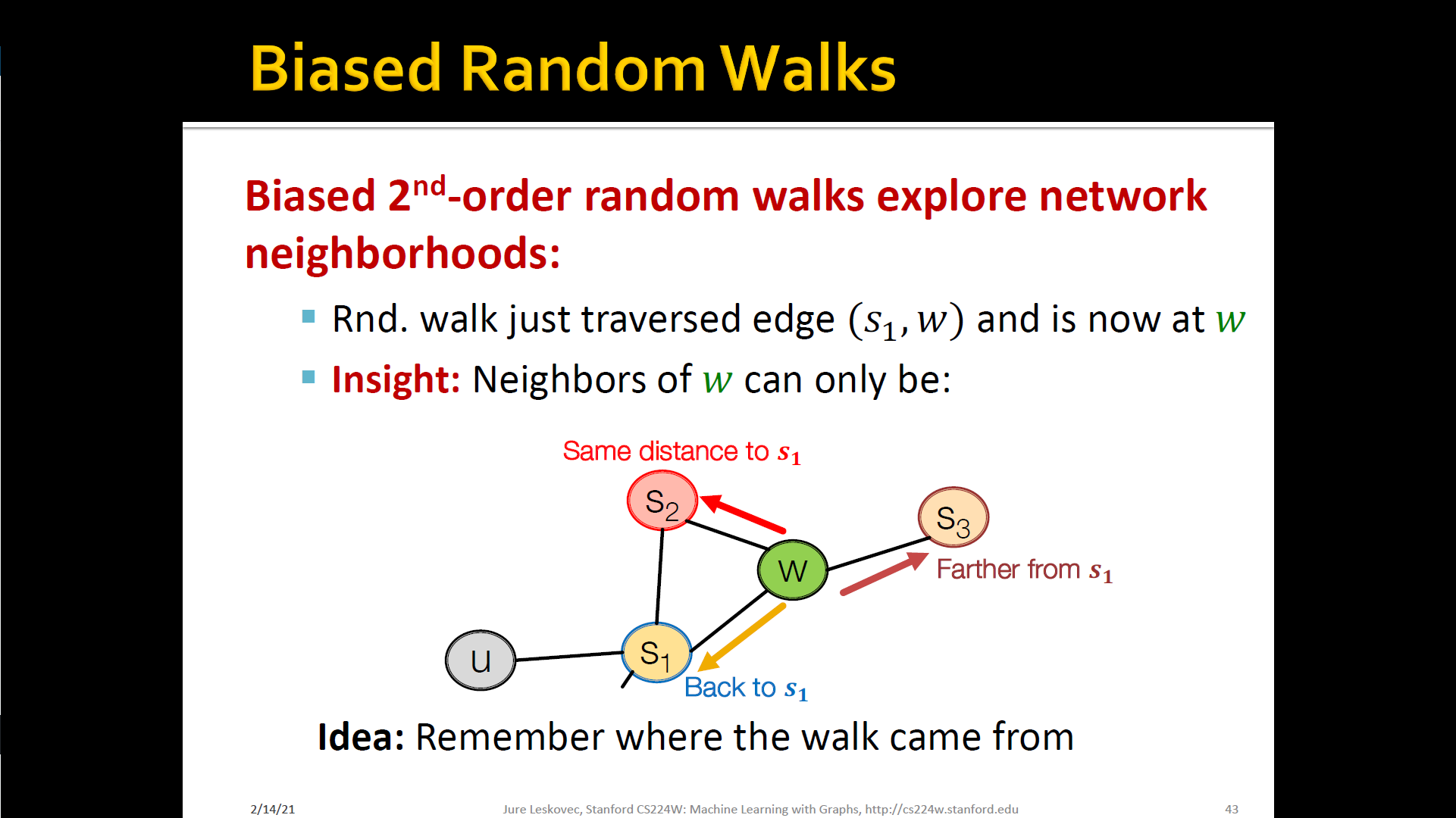
      • Return parameter $p$: Return back to the previous node
      • In-out parameter $q$: Moving outwards(DFS) vs. Inwards(BFS)
      • Intuitively, $q$ is the "ratio" of DFS vs. BFS

• Biased random walks

  • 

• Node2Vec algorihthm
  1. Compute random walk probabilities
  2. Simulate $r$ random walks of length $l$ starting from each node $u$
  3. Optimize the Node2Vec objective using Stochastic Gradient Descent
  • Linear-time complexity
  • All 3 steps are individually parallelizable
• Other random walk ideas
  • Different kinds of biased random walks
    • Based on node attributes
    • Based on learned weights
  • Alternative optimization schemes
    • Directly optimize based on 1-hop and 2-hop random walk probabilities
  • Network pre-processing techniques
    • Run random walks on modified versions of the original network

Summary

3.3 Embedding entire graphs

• Graph embedding $z_G$: Want to embed a subgraph or an entire graph $G$
• Tasks
  • Classifying toxic vs. non-toxic molecules
  • Identifying anomalous graphs

• Approach 1
  • Run a standard node embedding technique on the (sub) graph $G$
  • Then just sum (or average) the node embeddings in the (sub) graph $G$
    $z_G = \sum_{v \in G} z_v$
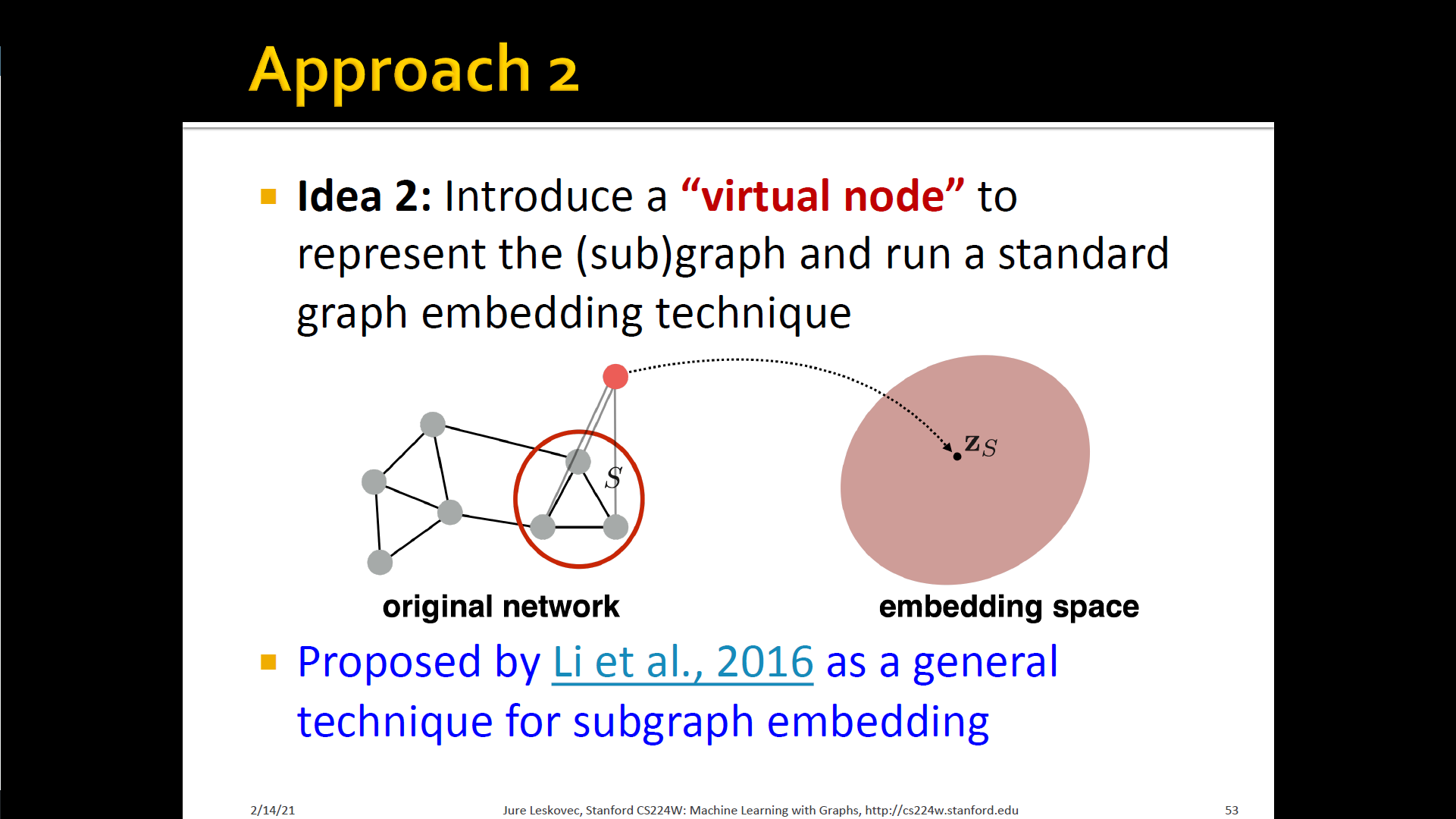
• Approach 2
  • Introduce a "virtual node" to represent the (sub) grpah and run a standard node embedding technique
    

• Approach 3 : Anonymous walk embeddings

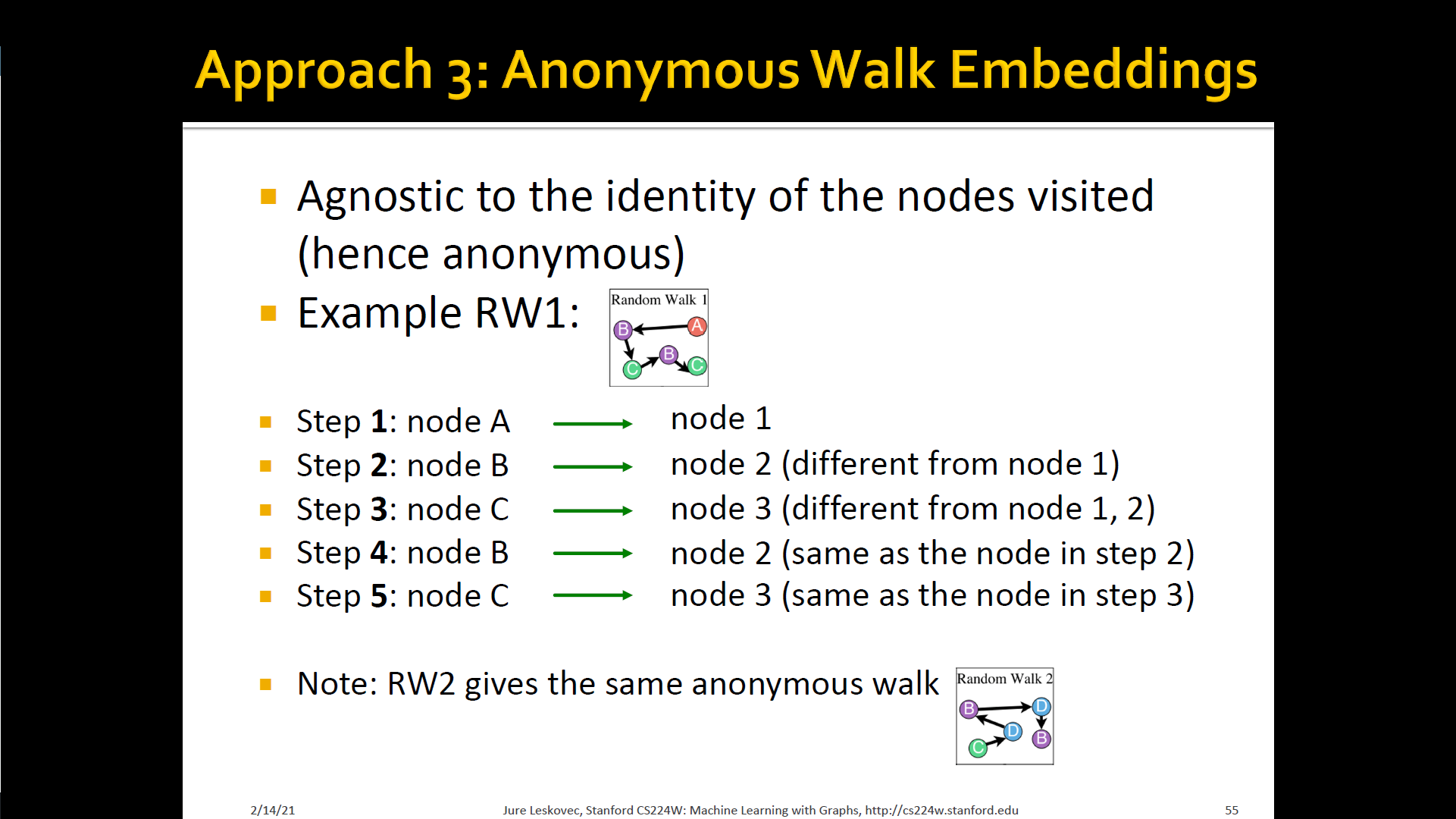
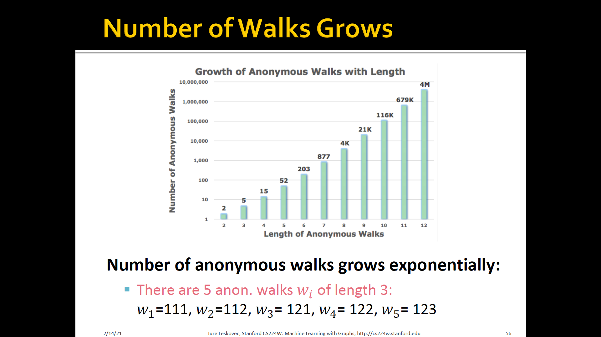
  • States in anonymous walks correspond to the index of the first time we visited the node in a random walk
    
    
    
    
    

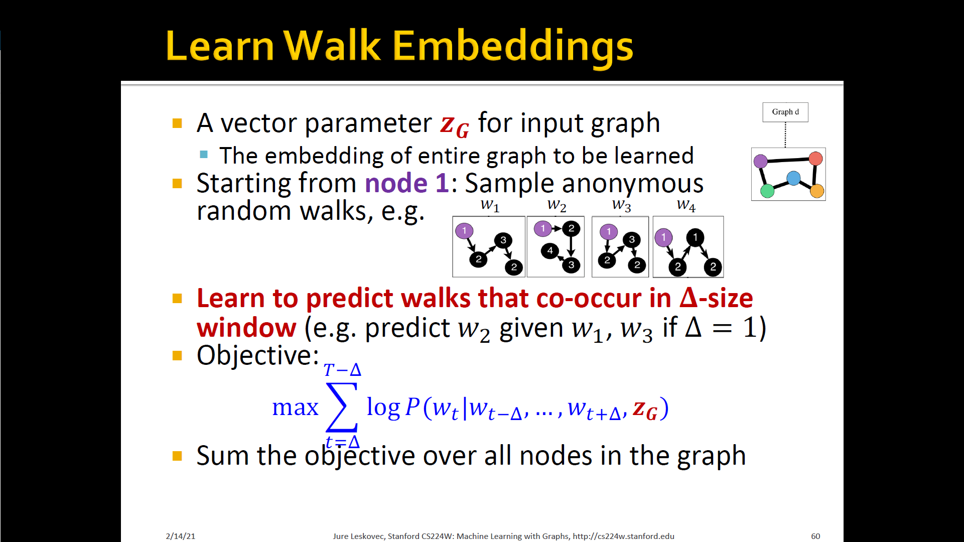
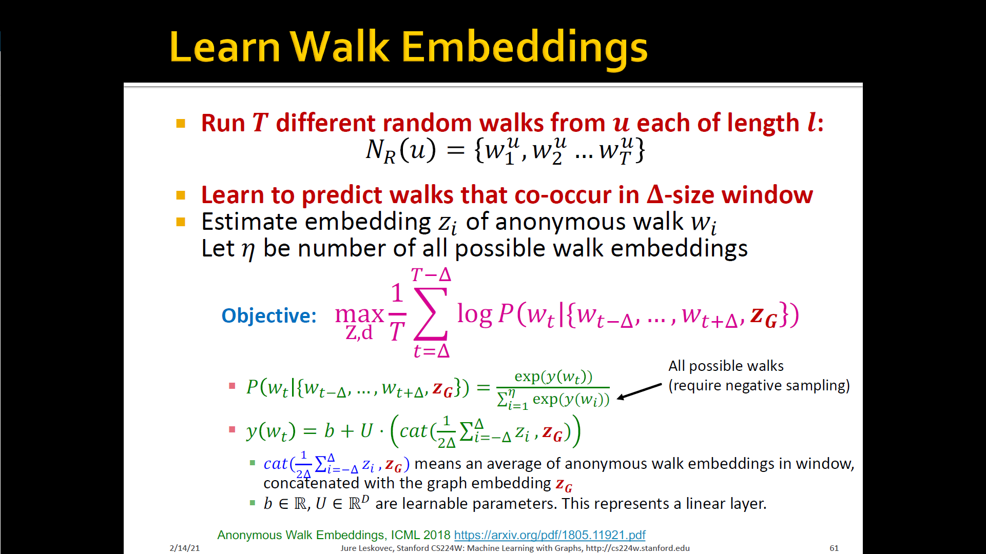
• New idea: Learn walk embeddings

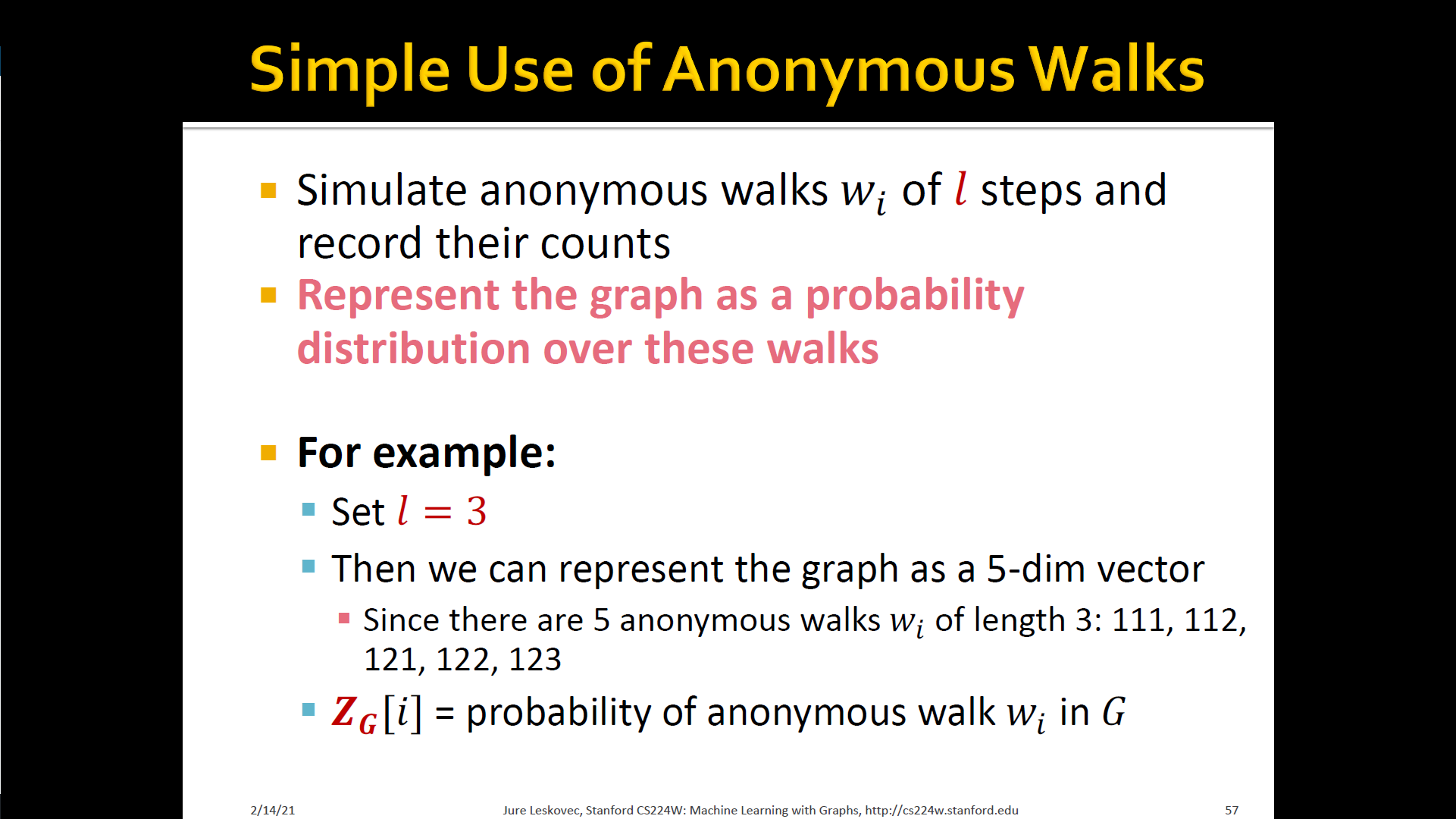
  • Rather than simply represent each walk by the fraction of times it occurs, we learn embedding $z_i$ of anonymous walk $w_i$
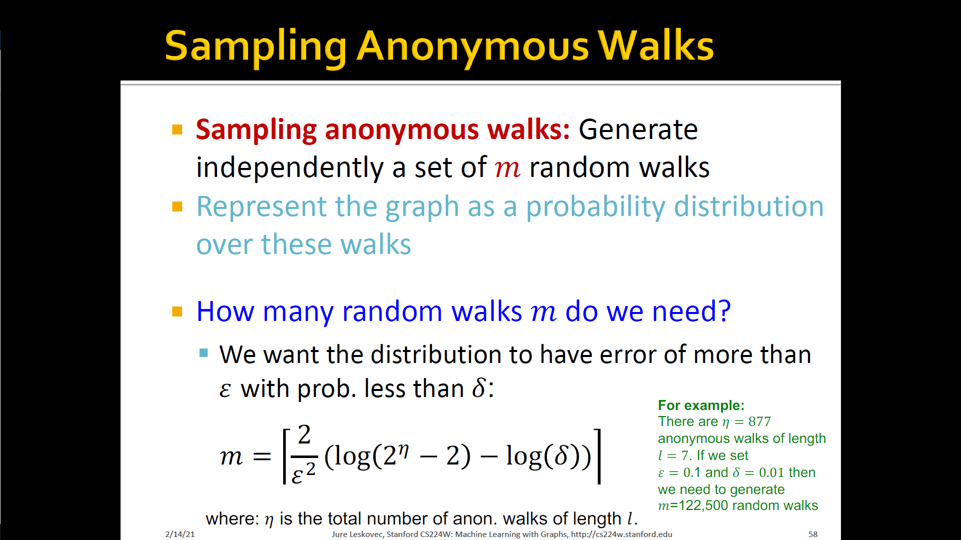
  • Learn a graph embedding $Z_G$ together with all the anonymous walk embeddings $z_i$. $Z={z_i:i=1, ..., \eta}$, where $\eta$ is the number of sampled anonymous walks
  • How to embed walks? Embed walks s.t. the next walk can be predicted

Summary

• How to use embeddings
  • Clustering/community detection: cluster points $z_i$
  • Node classification: Predict label of node $i$ based on $z_i$
  • Link prediction: Predict edge $(i, j)$ based on $(z_i, z_j)$
    • Where we can: concatenate, avg, product, or take a difference b/t the embeddings
  • Graph classification: graph embedding $z_G$ via aggregating node embeddings or anonymous random walks → Predict label based on graph embdding $z_G$

Summary