tensorflow의 기초에 대해서 배우고 있다.
tensorflow는 다양한 작업에 대해 데이터 흐름 프로그래밍을 위한 오픈소스 소프트웨어 라이브러리이다. 또한 추상화에 있고 디버깅과 시각화에 매우 능한 플랫폼입니다.그래서 많은 사람들이 딥러닝 혹은 머신러닝을 할 때 텐서플로우를 자주 사용한다.
텐서플로우를 활용한 linear regression!
import할 코드
import tensorflow as tf
import matplotlib.pyplot as plt

tf.random.set_seed(777)
tf에는 seed가 필요하다.
seed란 시작 숫자를 시드(seed)라고 한다. 일단 생성된 난수는 다음번 난수 생성을 위한 시드값이 된다. 따라서 시드값은 한 번만 정해주면 된다. 시드는 보통 현재 시각등을 이용하여 자동으로 정해지지만 사람이 수동으로 설정할 수도 있다. 특정한 시드값이 사용되면 그 다음에 만들어지는 난수들은 모두 예측할 수 있다.
가상 데이터셋
lr = 0.03

W_true = 3.0
B_true = 2.0


X = tf.random.normal((500, 1))
noise = tf.random.normal((500, 1))
y = X * W_true + B_true + noise


plt.scatter(X, y)
plt.show()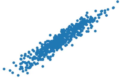
x,y의 scatter를 보면 그래프가 일정하다는 것을 볼 수 있다.
변수는 tf.Variable 클래스를 통해 생성 및 추적됩니다. tf.Variable은 ops를 실행하여 값을 변경할 수 있는 텐서를 나타냅니다.
텐서플로 홈페이지에 친절하게 설명되어있다. 변수를 생성하기 위해서는 tf.Variable()을 사용해주어야 한다.
w = tf.Variable(5.)
b = tf.Variable(0.)
w_records = [w.numpy()]
b_records = [b.numpy()]
loss_records = []
for epoch in range(100):
with tf.GradientTape() as tape:
y_hat = X * w + b
loss = tf.reduce_mean(tf.square((y - y_hat)))
dw, db = tape.gradient(loss, [w, b])
w.assign_sub(lr * dw)
b.assign_sub(lr * db)
w_records.append(w.numpy())
b_records.append(b.numpy())
loss_records.append(loss.numpy())어떻게 변하는가에 대해 알아볼 수 있도록 assign_sub를 활용해주자
이후 loss, w, b를 plt을 통해 시각화를 해보려고 한다.
plt.plot(loss_records)
plt.title('loss')
plt.show()
loss_records를 w_records와 b_records로 바꾸어주며 살펴보면 된다.
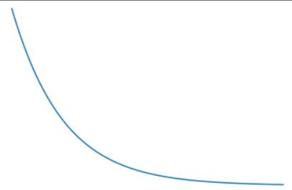

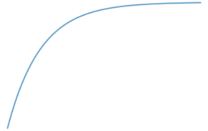
각각의 그래프를 확인할 수 있었다.
Dataset 당뇨병 진행도 예측하기
from sklearn.datasets import load_diabetes
import pandas as pd

diabetes = load_diabetes()
df = pd.DataFrame(diabetes.data, columns=diabetes.feature_names, dtype=np.float32)
df['const'] = np.ones(df.shape[0])
df.tail(3)를 Feature, ,를 가중치 벡터, 를 Target이라고 할 때,
의 역행령이 존재 한다고 가정했을 때,
아래의 식을 이용해 의 추정치 를 구해보자.
X = df
y = np.expand_dims(diabetes.target, axis=1).astype(np.float32)
XT = tf.transpose(X)
w = tf.matmul(tf.matmul(tf.linalg.inv(tf.matmul(XT, X)), XT), y)
y_pred = tf.squeeze(tf.matmul(X, w), axis=1)
print("예측한 진행도 :", y_pred[0].numpy(), "실제 진행도 :", diabetes.target[0])
print("예측한 진행도 :", y_pred[19].numpy(), "실제 진행도 :", diabetes.target[19])
print("예측한 진행도 :", y_pred[31].numpy(), "실제 진행도 :", diabetes.target[31])예측한 진행도 : 206.1170700734071 실제 진행도 : 151.0
예측한 진행도 : 124.01702486163391 실제 진행도 : 168.0
예측한 진행도 : 69.47588445588677 실제 진행도 : 59.0
텐서플로우 내 자체 데이터셋을 활용해서 선형 회귀에 대해서 알아볼 수 있었다.