상점의 아이템 수요예측
데이터
- Store(1,2,3), Item(1,2,3,...), Sales
EDA
- Store 별 Seasonality 체크
- EDA 결과로 적절한 Modeling 선택 가능
Modeling
-
Moving Average
-
Exponential Smoothing
- alpha 조절 잘 해야함 (grid search 관점으로 가도 괜찮을듯)
-
Double Exponential Smoothing
- 식 복잡..ㅋㅋ 나중에 찾아보기
-
Prophet
-
Box-cox
-
ARIMA
FB-prophet
개념
- Time-series forecasting model
- Missing data, shifts in the trend, outlier 에 강함
- 다양한 domain knowledge 에 적용 가능
- trend 가 비선형인 데이터(연도별, 주별, 일별, holiday)에서 자동으로 그 데이터의 변화 포인트를 찍어줌
- 연도별 seasonal component 에는 Fourier series 사용
- 주차별 seasonal component 에는 dummy variables 사용
- important holiday 알려주면 좋음
- g(t) = 부분선형 인 부분 혹은 logistic growth curve(exponential growth) in non-periodic changes in time series
- s(t) = periodic changes( weekly/yearly seasonality)P = 365.25(for yearly data), 7(for weekly data)
a_n, b_n = model seasonality - h(t) = 연휴 혹은 irregular schedule
- εt = unusual change 로 부터 나오는 error
- 즉, non-linear, linear 섞여있을때 regressor 로 fit 해줌
- 시간적 데이터보다 curve 에 더 의존적 인 모델
- Upper bound, lower bound 설정
- 변곡점 잘 세팅해주는게 포인트(business insight 중요)
코드 예시
- 상황: digital marketing platform 광고 소비 데이터(fake data 숨겨져있음),
17개월 데이터로 다음 30일 ad spend 예측(2017-06-01~2018-12-30, 577rows, 2columns(date and spend))
from fbprophet import Prophet
sample = pd.read_csv(data위치)
model2=Prophet( interval_width=0.95,
		yearly_seasonality=True,
        	weekly_seasonality=True,
        	holidays=us_public_holidays,
        	changepoint_prior_scale=2)
model2.add_seasonality(name=’monthly’, period=30.5, fourier_order=5, prior_scale=0.02)
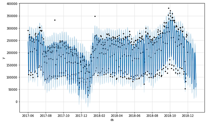
-> black dots : real data, deep blue line: forecasting numbers, light blue: 95% c.i.
- MAPE or MAE 로 error 측정
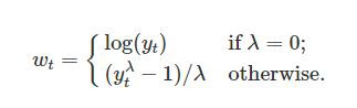
Box-Cox Transformation
개념
- Transformations can cut away white noise(Normal distribution으로 만들어줌)
- non-time series data에서도 사용 가능

t = time, lambda = parameter we choose - lambda 는 어떻게 설정할까?
- best normal distribution 을 만들어주는걸로
scipy.special.inv_boxcox(y, lambda)- Box-Cox transformation 의 한계: 해석이 중요한 경우에는 안 좋은 선택
- 결국 y값을 normalization 해주는 느낌 (아래 코드 참고)
train_df2['y'], lambda_prophet = stats.boxcox(train_df2['y'])
train_df2.reset_index(inplace=True)
%%time
m2 = Prophet(yearly_seasonality=True, weekly_seasonality=True, daily_seasonality=True)
m2.fit(train_df2[['ds','y']]);
ARIMA
- Non-stationary(constant mean (x), constant variance (x), autocovariance depend on time)
- trend, seasonality 제거하는 방법
- Transformation (log, sqrt...)
- Differencing
- Smoothing (rolling avg...)
- Decomposition
- Polynomial Fitting (fit a regression model)

사진 출처: https://www.slideshare.net/21_venkat?
- AR(Auto Regression) : 이전 데이터를 기반으로 다음 스텝 예측(linear function)
- I (Integration) : stationary 를 만들기 위해
- MA (Moving Average) : 이전 데이터 평균으로 예측
p, d, q 어떻게 결정할까?
- p 를 결정하기 위해 PACF 사용
- q 를 결정하기 위해 ACF 사용
SARIMA (ARIMA + Seasonality)
-
log, diff(1) 을 통해 stationary 하게 만듬

-> log
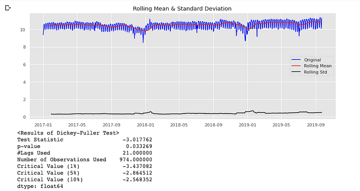
-> diff

-
code
import statsmodels.api as sm
fit1 = sm.tsa.statespace.SARIMAX(train.Spend, order=(7, 1, 2), seasonal_order=(0, 1, 2, 7)).fit(use_boxcox=True)
test['SARIMA'] = fit1.predict(start="2019-07-23", end="2019-09-23", dynamic=True)
plt.figure(figsize=(16, 8))
plt.plot(train['Spend'], label='Train')
plt.plot(test['Spend'], label='Test')
plt.plot(test['SARIMA'], label='SARIMA')
plt.legend(loc='best')
plt.show()
Holt-Winter's Seasonal Smoothing(one of exponential smoothing)
from statsmodels.tsa.api import ExponentialSmoothing
fit1 = ExponentialSmoothing(np.asarray(train['Spend']) ,seasonal_periods=7 ,trend='add', seasonal='add').fit(use_boxcox=True)
test['Holt_Winter'] = fit1.forecast(len(test))
plt.figure(figsize=(16,8))
plt.plot( train['Spend'], label='Train')
plt.plot(test['Spend'], label='Test')
plt.plot(test['Holt_Winter'], label='Holt_Winter')
plt.legend(loc='best')
plt.show()
Data Scientist or Gourmet