BERT: Pre-training of Deep Bidirectional Transformers for Language Understanding 논문 번역
Abstract
We introduce a new language representation
우리는 새로운 언어 표현 모델인 BERT를 소개합니다.
****model called BERT, which stands for Bidirectional Encoder Representations from Transformers.
BERT는 Bidirectional Encoder Representations from Transformers의 약자입니다.
Unlike recent language representation models (Peters et al., 2018a; Radford et al., 2018), BERT is designed to pretrain deep bidirectional representations from unlabeled text by jointly conditioning on both left and right context in all layers.
기존의 언어 표현 모델들(Peters et al., 2018a; Radford et al., 2018)과 달리, BERT는 모든 층에서 좌우(양방향) 문맥을 동시에 고려하여 비지도(unlabeled) 텍스트로부터 깊이 있는 양방향 표현을 사전 학습(pretrain)하도록 설계되었습니다.
As a result, the pre-trained BERT model can be finetuned with just one additional output layer to create state-of-the-art models for a wide range of tasks, such as question answering and language inference, without substantial taskspecific architecture modifications.
이러한 사전 학습 덕분에 BERT는 단 하나의 출력 레이어만 추가하여 질의응답(question answering), 문장 추론(language inference) 등 다양한 작업에서 최첨단(state-of-the-art) 성능을 달성할 수 있습니다. 특히, 별도의 복잡한 작업별 아키텍처 수정 없이 손쉽게 미세 조정(fine-tuning)이 가능합니다.
BERT is conceptually simple and empirically powerful.
BERT는 개념적으로 단순하지만 실험적으로 매우 강력합니다.
It obtains new state-of-the-art results on eleven natural language processing tasks, including pushing the GLUE score to 80.5% (7.7% point absolute improvement), MultiNLI accuracy to 86.7% (4.6% absolute improvement), SQuAD v1.1 question answering Test F1 to 93.2 (1.5 point absolute improvement) and SQuAD v2.0 Test F1 to 83.1 (5.1 point absolute improvement).
BERT는 총 11개의 자연어 처리(NLP) 작업에서 새로운 최고 성능을 기록했으며, 다음과 같은 눈에 띄는 개선을 보였습니다:
- GLUE 점수: 80.5% (절대 7.7%p 향상)
- MultiNLI 정확도: 86.7% (절대 4.6%p 향상)
- SQuAD v1.1 질의응답 테스트 F1 점수: 93.2 (절대 1.5%p 향상)
- SQuAD v2.0 테스트 F1 점수: 83.1 (절대 5.1%p 향상)
1 Introduction
Language model pre-training has been shown to be effective for improving many natural language processing tasks (Dai and Le, 2015; Peters et al., 2018a; Radford et al., 2018; Howard and Ruder, 2018).
언어 모델의 사전 학습(language model pre-training)은 여러 자연어 처리 작업(NLP tasks)의 성능 향상에 효과적인 것으로 입증되었습니다(Dai & Le, 2015; Peters et al., 2018a; Radford et al., 2018; Howard & Ruder, 2018).
These include sentence-level tasks such as natural language inference (Bowman et al., 2015; Williams et al., 2018) and paraphrasing (Dolan and Brockett, 2005), which aim to predict the relationships between sentences by analyzing them holistically, as well as token-level tasks such as
named entity recognition and question answering, where models are required to produce fine-grained output at the token level (Tjong Kim Sang and De Meulder, 2003; Rajpurkar et al., 2016).
이러한 작업에는 문장 수준의 작업(sentence-level tasks)과 토큰 수준의 작업(token-level tasks)이 포함됩니다.
문장 수준 작업에는 자연어 추론(NLI, Natural Language Inference) (Bowman et al., 2015; Williams et al., 2018)이나 문장 패러프레이징(paraphrasing) (Dolan & Brockett, 2005) 등이 있으며, 이는 두 문장 간의 관계를 전체적으로 분석하여 예측하는 작업입니다.
토큰 수준 작업으로는 개체명 인식(NER, Named Entity Recognition) (Tjong Kim Sang & De Meulder, 2003)과 질의응답(Question Answering) (Rajpurkar et al., 2016) 등이 있으며, 이 경우 모델은 토큰 단위에서 세밀한 출력을 생성해야 합니다.
There are two existing strategies for applying pre-trained language representations to downstream tasks: feature-based and fine-tuning.
사전 학습된 언어 표현을 다운스트림 작업에 적용하는 방법에는 두 가지 전략이 있습니다:
The feature-based approach, such as ELMo (Peters et al., 2018a), uses task-specific architectures that include the pre-trained representations as additional features.
첫번째로 Feature-based 접근법, 대표적으로 ELMo(Peters et al., 2018a)가 있으며, 이는 사전 학습된 표현을 추가적인 입력 피처로 사용하는 작업별(task-specific) 아키텍처를 설계하여 사용합니다.
The fine-tuning approach, such as the Generative Pre-trained Transformer (OpenAI GPT) (Radford et al., 2018), introduces minimal task-specific parameters, and is trained on the downstream tasks by simply fine-tuning all pretrained parameters.
두번째로 Fine-tuning 접근법, OpenAI GPT(Radford et al., 2018)와 같은 방식으로, 최소한의 작업별 매개변수를 추가한 후, 사전 학습된 모든 파라미터를 다운스트림 작업에 맞춰 미세 조정합니다.
The two approaches share the same objective function during pre-training, where they use unidirectional language models to learn general language representations.
이 두 접근법은 공통적으로 사전 학습 중에는 단방향 언어 모델(unidirectional language models) 을 사용하여 일반적인 언어 표현을 학습한다는 점을 공유합니다.
We argue that current techniques restrict the power of the pre-trained representations, especially
for the fine-tuning approaches.
하지만 우리는 이러한 기존 기술이 특히 fine-tuning 방식 에서 사전 학습 표현의 강력함을 충분히 활용하지 못하도록 제한한다고 주장합니다.
The major limitation is that standard language models are unidirectional, and this limits the choice of architectures that can be used during pre-training.
그 가장 큰 한계는 표준 언어 모델이 단방향(unidirectional) 이라는 점입니다.
이로 인해 사전 학습 중 사용할 수 있는 아키텍처에 제약이 생깁니다.
For example, in OpenAI GPT, the authors use a left-toright architecture, where every token can only attend to previous tokens in the self-attention layers of the Transformer (Vaswani et al., 2017).
예를 들어, OpenAI GPT 에서는 왼쪽에서 오른쪽으로만(LTR) 정보를 처리하는 아키텍처를 사용합니다. 이는 트랜스포머(Transformer) 모델의 self-attention 레이어에서 각 토큰이 자신보다 이전에 나온 토큰들만 주목(attend)할 수 있도록 제한합니다(Vaswani et al., 2017).
Such restrictions are sub-optimal for sentence-level tasks, and could be very harmful when applying finetuning based approaches to token-level tasks such as question answering, where it is crucial to incorporate context from both directions.
이러한 제한은 문장 수준의 작업 에는 비효율적일 뿐 아니라, 질의응답과 같은 토큰 수준 작업 에서는 매우 치명적일 수 있습니다.
왜냐하면 이러한 작업에서는 양방향으로 문맥을 통합해 이해하는 것 이 필수적이기 때문입니다.
In this paper, we improve the fine-tuning based approaches by proposing BERT: Bidirectional
Encoder Representations from Transformers.
본 논문에서 우리는 BERT(Bidirectional Encoder Representations from Transformers) 를 제안하여 기존의 fine-tuning 기반 접근법을 개선합니다.
BERT alleviates the previously mentioned unidirectionality constraint by using a “masked language
model” (MLM) pre-training objective, inspired by the Cloze task (Taylor, 1953).
BERT는 앞서 언급한 단방향(unidirectionality)의 한계를 “마스크드 언어 모델(Masked Language Model, MLM)” 이라는 사전 학습 목표를 통해 해결합니다. 이 방법은 클로즈(Cloze) 테스트(Taylor, 1953)에서 영감을 받았습니다.
The masked language model randomly masks some of the tokens from the input, and the objective is to predict the original vocabulary id of the masked word based only on its context. Unlike left-toright language model pre-training, the MLM objective enables the representation to fuse the left
and the right context, which allows us to pretrain a deep bidirectional Transformer.
마스크드 언어모델은 입력 문장에서 일부 토큰을 무작위로 마스킹한 후, 주변 문맥 정보만으로 해당 마스킹된 단어의 원래 단어를 예측하도록 학습합니다. 기존의 왼쪽에서 오른쪽(LTR) 언어 모델과는 달리, 이 MLM 방식은 좌우 양방향 문맥을 통합(fuse) 할 수 있게 만들어, 깊은 양방향 트랜스포머를 사전 학습할 수 있도록 합니다.
In addition to the masked language model, we also use a “next sentence prediction” task that jointly pretrains text-pair representations.
또한, 마스크드 언어 모델 외에도 “다음 문장 예측(Next Sentence Prediction, NSP)” 작업을 추가하여 문장 쌍(Text pair) 의 관계를 공동으로 학습하도록 설계했습니다.
The contributions of our paper are as follows:
본 논문의 주요 기여는 다음과 같습니다.
- We demonstrate the importance of bidirectional pre-training for language representations. 양방향 사전 학습의 중요성을 입증했습니다. Unlike Radford et al. (2018), which uses unidirectional language models for pre-training, BERT
uses masked language models to enable pretrained deep bidirectional representations. 기존의 Radford et al. (2018) 은 단방향 언어 모델을 사용했으나, BERT는 마스크드 언어 모델을 활용하여 깊이 있는 양방향 표현을 사전 학습합니다. This is also in contrast to Peters et al. (2018a), which uses a shallow concatenation of independently
trained left-to-right and right-to-left LMs. 이는 Peters et al. (2018a) 의 방식(좌우 각각 독립적으로 학습한 모델의 얕은 결합)과도 차별화됩니다.
- We show that pre-trained representations reduce the need for many heavily-engineered taskspecific architectures. 사전 학습된 표현(pre-trained representations) 을 통해 복잡하게 설계된 작업별 맞춤형 아키텍처(task-specific architectures) 의 필요성을 줄일 수 있음을 보여줍니다. BERT is the first finetuning based representation model that achieves state-of-the-art performance on a large suite of sentence-level and token-level tasks, outperforming many task-specific architectures. BERT는 fine-tuning 기반의 표현 모델로서, 문장 수준과 토큰 수준의 다양한 과제에서 최첨단 성능을 최초로 달성했으며, 여러 복잡한 작업별 설계보다 우수한 결과를 보였습니다.
- BERT advances the state of the art for eleven NLP tasks. BERT는 총 11가지 NLP 과제에서 기존 최고 성능을 뛰어넘는 결과를 냈습니다. The code and pre-trained models are available at https://github.com/ google-research/bert. 코드 및 사전 학습 모델은 아래 링크에서 사용할 수 있습니다: https://github.com/google-research/bert
2 Related Work
There is a long history of pre-training general language representations, and we briefly review the most widely-used approaches in this section.
일반적인 언어 표현을 사전 학습하는 연구는 오랜 역사를 가지고 있으며, 이 절에서는 가장 널리 사용되는 접근 방식을 간략히 살펴봅니다.
2.1 Unsupervised Feature-based Approaches
2.1 비지도(feature-based) 방식 접근법
Learning widely applicable representations of words has been an active area of research for decades, including non-neural (Brown et al., 1992; Ando and Zhang, 2005; Blitzer et al., 2006) and neural (Mikolov et al., 2013; Pennington et al., 2014) methods.
다양한 분야에서 사용할 수 있는 단어 표현을 학습하는 연구는 수십 년간 활발히 진행되어 왔으며, 여기에는 비신경망(non-neural) 방식과 신경망(neural) 방식이 모두 포함됩니다.
Pre-trained word embeddings are an integral part of modern NLP systems, offering significant improvements over embeddings learned from scratch (Turian et al., 2010).
사전 학습된 단어 임베딩은 현대 자연어 처리 시스템의 핵심 요소로, 처음부터 학습한 임베딩에 비해 큰 성능 향상을 제공합니다.
To pre-train word embedding vectors, left-to-right language modeling objectives have been used (Mnih and Hinton, 2009), as well as objectives to discriminate correct from incorrect words in left and right context (Mikolov et al., 2013).
단어 임베딩 벡터를 사전 학습하기 위해 주로 왼쪽에서 오른쪽으로 진행하는 언어 모델링 목표가 사용되었으며, 왼쪽 및 오른쪽 문맥 내에서 올바른 단어와 잘못된 단어를 구별하는 목적 또한 사용되었습니다.
These approaches have been generalized to coarser granularities, such as sentence embeddings (Kiros et al., 2015; Logeswaran and Lee, 2018) or paragraph embeddings (Le and Mikolov, 2014).
이러한 접근 방식은 더 큰 단위인 문장 임베딩이나 단락 임베딩으로 일반화되었습니다.
To train sentence representations, prior work has used objectives to rank candidate next sentences (Jernite et al., 2017; Logeswaran and Lee, 2018), left-to-right generation of next sentence words given a representation of the previous sentence (Kiros et al., 2015), or denoising autoencoder derived objectives (Hill et al., 2016).
문장 표현을 학습하기 위해, 이전 연구에서는 다음 문장의 후보 순위를 매기는 방식, 이전 문장을 바탕으로 다음 문장을 왼쪽에서 오른쪽으로 생성하는 방식, 또는 디노이징 오토인코더 기반 목표를 사용했습니다.
ELMo and its predecessor (Peters et al., 2017, 2018a) generalize traditional word embedding research along a different dimension.
ELMo와 그 이전 모델은 기존 단어 임베딩 연구를 다른 차원으로 확장했습니다.
They extract context-sensitive features from a left-to-right and a right-to-left language model.
이들은 왼쪽에서 오른쪽, 오른쪽에서 왼쪽으로 학습된 언어 모델에서 문맥에 민감한 특징을 추출합니다.
The contextual representation of each token is the concatenation of the left-to-right and right-to-left representations.
각 토큰의 문맥 표현은 양방향 모델의 출력을 단순히 이어 붙인(concatenate) 형태입니다.
When integrating contextual word embeddings with existing task-specific architectures, ELMo advances the state of the art for several major NLP benchmarks (Peters et al., 2018a) including question answering (Rajpurkar et al., 2016), sentiment analysis (Socher et al., 2013), and named entity recognition (Tjong Kim Sang and De Meulder, 2003).
이러한 ELMo 임베딩을 기존 작업 특화 아키텍처에 결합하면, 질의응답, 감정 분석, 개체명 인식 등 다양한 주요 NLP 벤치마크에서 최첨단 성능을 기록할 수 있었습니다.
Melamud et al. (2016) proposed learning contextual representations through a task to predict a single word from both left and right context using LSTMs.
Melamud 등(2016)은 양방향 문맥을 활용해 하나의 단어를 예측하는 작업을 통해 문맥적 표현을 학습하는 방법을 제안했습니다.
Similar to ELMo, their model is feature-based and not deeply bidirectional.
이 모델도 ELMo와 마찬가지로 feature-based 방식이며, 깊은 양방향성을 갖춘 모델은 아닙니다.
Fedus et al. (2018) shows that the cloze task can be used to improve the robustness of text generation models.
Fedus 등(2018)은 클로즈(cloze) 작업이 텍스트 생성 모델의 견고함을 높이는 데 활용될 수 있음을 보여주었습니다.
2.2 Unsupervised Fine-tuning Approaches
2.2 비지도 학습 기반 미세 조정(Fine-tuning) 접근법
As with the feature-based approaches, the first works in this direction only pre-trained word embedding parameters from unlabeled text (Collobert and Weston, 2008).
feature-based 방식과 마찬가지로, 초기 연구는 비지도(unlabeled) 텍스트로부터 단어 임베딩 파라미터만 사전 학습하는 데 집중했습니다.
More recently, sentence or document encoders which produce contextual token representations have been pre-trained from unlabeled text and fine-tuned for a supervised downstream task (Dai and Le, 2015; Howard and Ruder, 2018; Radford et al., 2018).
최근에는 문장 또는 문서 인코더가 비지도 데이터로부터 사전 학습되고, 이를 감독 학습이 필요한 다운스트림 작업에 맞게 미세 조정하는 방식이 주목받고 있습니다.
The advantage of these approaches is that few parameters need to be learned from scratch.
이러한 방식의 장점은 처음부터 새로 학습해야 할 파라미터의 수가 매우 적다는 점입니다.
At least partly due to this advantage, OpenAI GPT (Radford et al., 2018) achieved previously state-of-the-art results on many sentence-level tasks from the GLUE benchmark (Wang et al., 2018a).
이러한 이점 덕분에 OpenAI GPT는 GLUE 벤치마크의 다양한 문장 수준 작업에서 이전 최고 성능을 달성할 수 있었습니다.
Left-to-right language modeling and auto-encoder objectives have been used for pre-training such models (Howard and Ruder, 2018; Radford et al., 2018; Dai and Le, 2015).
이러한 모델의 사전 학습에는 왼쪽에서 오른쪽으로 진행하는 언어 모델링과 오토인코더(auto-encoder) 기반 목표가 주로 사용되었습니다.
2.3 Transfer Learning from Supervised Data
2.3 감독 학습 데이터로부터의 전이 학습(Transfer Learning)
There has also been work showing effective transfer from supervised tasks with large datasets, such as natural language inference (Conneau et al., 2017) and machine translation (McCann et al., 2017).
또한 대규모 데이터셋을 사용하는 감독 학습 작업(예: 자연어 추론 및 기계 번역)에서 효과적인 전이 학습 사례도 보고되었습니다.
Computer vision research has also demonstrated the importance of transfer learning from large pre-trained models, where an effective recipe is to fine-tune models pre-trained with ImageNet (Deng et al., 2009; Yosinski et al., 2014).
컴퓨터 비전 분야 연구에서도 대규모 사전 학습 모델로부터의 전이 학습이 중요함이 입증되었으며, 대표적인 성공 사례는 ImageNet 으로 사전 학습된 모델을 미세 조정(fine-tune)하는 방법입니다.
3 BERT
3 BERT
We introduce BERT and its detailed implementation in this section.
이 절에서는 BERT와 그 구체적인 구현 방법을 소개합니다.
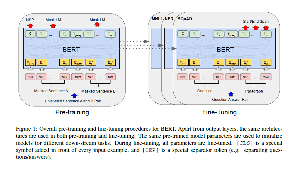
There are two steps in our framework: pre-training and fine-tuning.
우리의 프레임워크는 두 단계로 이루어져 있습니다: 사전 학습(pre-training)과 미세 조정(fine-tuning)입니다.
During pre-training, the model is trained on unlabeled data over different pre-training tasks.
사전 학습 단계에서는 레이블이 없는 데이터(unlabeled data)로 다양한 사전 학습 작업을 수행합니다.
For fine-tuning, the BERT model is first initialized with the pre-trained parameters, and all of the parameters are fine-tuned using labeled data from the downstream tasks.
미세 조정 단계에서는 사전 학습된 파라미터로 BERT 모델을 초기화하고, 다운스트림 작업의 레이블이 포함된 데이터를 사용해 모든 파라미터를 미세 조정합니다.
Each downstream task has separate fine-tuned models, even though they are initialized with the same pre-trained parameters.
모든 다운스트림 작업은 같은 사전 학습 파라미터로 시작하지만, 각 작업마다 별도의 미세 조정 모델을 가집니다.
The question-answering example in Figure 1 will serve as a running example for this section.
도표 1에 나오는 질의응답(question-answering) 예시는 이 절의 대표 사례로 사용됩니다.
A distinctive feature of BERT is its unified architecture across different tasks.
BERT의 특징 중 하나는 다양한 작업에 동일하게 적용 가능한 통합 아키텍처를 가지고 있다는 점입니다.
There is minimal difference between the pre-trained architecture and the final downstream architecture.
사전 학습 때의 모델 아키텍처와 다운스트림 작업에서의 최종 모델 아키텍처 사이에는 거의 차이가 없습니다.
Model Architecture
모델 아키텍처
BERT’s model architecture is a multi-layer bidirectional Transformer encoder based on the original implementation described in Vaswani et al. (2017) and released in the tensor2tensor library.
BERT의 모델 아키텍처는 Vaswani et al.(2017)에서 설명된 원래 구현을 기반으로 한 다층 양방향 트랜스포머 인코더이며, 이는 tensor2tensor 라이브러리에도 공개되어 있습니다.
Because the use of Transformers has become common and our implementation is almost identical to the original, we will omit an exhaustive background description of the model architecture and refer readers to Vaswani et al. (2017) as well as excellent guides such as “The Annotated Transformer.”
트랜스포머의 사용이 보편화되었고, 우리 구현 또한 원본과 거의 동일하므로, 아키텍처에 대한 자세한 설명은 생략하고 독자들에게 Vaswani et al.(2017) 및 “The Annotated Transformer”와 같은 훌륭한 참고 자료를 권장합니다.
In this work, we denote the number of layers (i.e., Transformer blocks) as L, the hidden size as H, and the number of self-attention heads as A.
이 논문에서 L은 레이어(트랜스포머 블록)의 개수, H는 히든 크기, A는 self-attention 헤드 수를 나타냅니다.
We primarily report results on two model sizes: BERTBASE (L=12, H=768, A=12, Total Parameters=110M) and BERTLARGE (L=24, H=1024, A=16, Total Parameters=340M).
우리는 주로 두 가지 모델 크기에서 실험 결과를 보고합니다: BERTBASE (L=12, H=768, A=12, 파라미터 1억 1천만 개)와 BERTLARGE (L=24, H=1024, A=16, 파라미터 3억 4천만 개)입니다.
BERTBASE was chosen to have the same model size as OpenAI GPT for comparison purposes.
BERTBASE는 OpenAI GPT와의 공정한 비교를 위해 유사한 모델 크기로 설정되었습니다.
Critically, however, the BERT Transformer uses bidirectional self-attention, while the GPT Transformer uses constrained self-attention where every token can only attend to context to its left.
하지만 중요한 차이점은, BERT의 트랜스포머는 양방향 self-attention 을 사용하고, GPT 트랜스포머는 왼쪽 방향으로만 context를 참조하는 제한적 self-attention 을 사용한다는 점입니다.
Input/Output Representations
입출력 표현 방식
To make BERT handle a variety of down-stream tasks, our input representation is able to unambiguously represent both a single sentence and a pair of sentences (e.g., <Question, Answer>) in one token sequence.
BERT가 다양한 다운스트림 작업을 처리할 수 있도록 하기 위해, 입력 표현은 한 개의 문장 또는 문장 쌍(예: <질문, 답변>)을 하나의 토큰 시퀀스 안에서 명확히 표현할 수 있습니다.
Throughout this work, a “sentence” can be an arbitrary span of contiguous text, rather than an actual linguistic sentence.
이 논문에서 말하는 "문장"은 실제 언어학적 문장이 아니라, 연속된 텍스트의 임의 구간을 의미합니다.
A “sequence” refers to the input token sequence to BERT, which may be a single sentence or two sentences packed together.
"시퀀스"는 BERT에 입력되는 토큰 시퀀스를 의미하며, 하나의 문장 또는 두 개의 문장이 함께 포함될 수 있습니다.
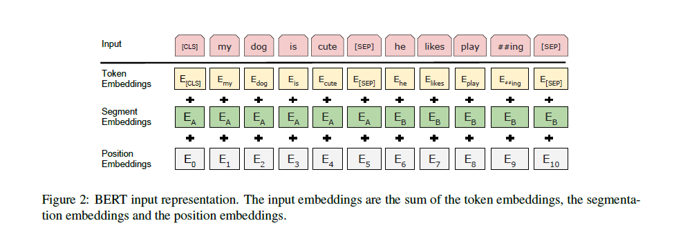
We use WordPiece embeddings (Wu et al., 2016) with a 30,000 token vocabulary.
우리는 WordPiece 임베딩(30,000개 토큰으로 구성된 어휘)를 사용합니다.
The first token of every sequence is always a special classification token ([CLS]).
모든 시퀀스의 첫 번째 토큰은 항상 특별한 분류 토큰([CLS])입니다.
The final hidden state corresponding to this token is used as the aggregate sequence representation for classification tasks.
이 [CLS] 토큰에 해당하는 최종 히든 상태는 분류 작업에서 전체 시퀀스를 대표하는 벡터로 사용됩니다.
Sentence pairs are packed together into a single sequence.
두 문장은 하나의 시퀀스 안에 함께 결합됩니다.
We differentiate the sentences in two ways.
두 문장을 구분하는 방법은 두 가지입니다.
First, we separate them with a special token ([SEP]).
첫째, 두 문장을 [SEP]라는 특별한 구분 토큰으로 나눕니다.
Second, we add a learned embedding to every token indicating whether it belongs to sentence A or sentence B.
둘째, 각 토큰이 문장 A에 속하는지 문장 B에 속하는지 알려주는 학습된 구분 임베딩(segment embedding)을 추가합니다.
As shown in Figure 1, we denote input embedding as E, the final hidden vector of the special [CLS] token as C ∈ RH, and the final hidden vector for the ith input token as Ti ∈ RH.
그림 1에서와 같이, 입력 임베딩을 E로 표기하고, [CLS] 토큰의 최종 히든 벡터는 C ∈ RH, i번째 입력 토큰의 최종 히든 벡터는 Ti ∈ RH로 표기합니다.
For a given token, its input representation is constructed by summing the corresponding token, segment, and position embeddings.
각 토큰의 입력 표현은 해당 토큰 임베딩, 세그먼트 임베딩, 포지션 임베딩을 합쳐서 구성됩니다.
A visualization of this construction can be seen in Figure 2.
이 입력 표현 방식의 시각적 설명은 그림 2에서 확인할 수 있습니다.
3.1 Pre-training BERT
3.1 BERT의 사전 학습
Unlike Peters et al. (2018a) and Radford et al. (2018), we do not use traditional left-to-right or right-to-left language models to pre-train BERT.
Peters et al.(2018a)와 Radford et al.(2018)과는 달리, 우리는 전통적인 왼쪽-오른쪽 또는 오른쪽-왼쪽 언어 모델을 사용하여 BERT를 사전 학습하지 않습니다.
Instead, we pre-train BERT using two unsupervised tasks, described in this section.
대신, 이 절에서 설명하는 두 가지 비지도 학습 과제를 통해 BERT를 사전 학습합니다.
This step is presented in the left part of Figure 1.
이 단계는 그림 1의 왼쪽 부분에 나타나 있습니다.
Task #1: Masked LM
과제 #1: 마스크드 언어 모델(MLM)
Intuitively, it is reasonable to believe that a deep bidirectional model is strictly more powerful than either a left-to-right model or the shallow concatenation of a left-to-right and a right-to-left model.
직관적으로 보면, 깊은 양방향 모델이 왼쪽-오른쪽 모델이나 얕게 결합된 좌우 단방향 모델보다 훨씬 강력하다고 보는 것이 타당합니다.
Unfortunately, standard conditional language models can only be trained left-to-right or right-to-left, since bidirectional conditioning would allow each word to indirectly “see itself,” and the model could trivially predict the target word in a multi-layered context.
그러나 표준 조건부 언어 모델은 각 단어가 자기 자신을 간접적으로 볼 수 있게 되어 목표 단어를 너무 쉽게 예측하는 문제가 생기므로, 오직 한 방향(왼쪽-오른쪽 또는 오른쪽-왼쪽)으로만 훈련할 수 있습니다.
In order to train a deep bidirectional representation, we simply mask some percentage of the input tokens at random, and then predict those masked tokens.
이러한 깊은 양방향 표현을 학습하기 위해, 우리는 입력 토큰 중 일부를 무작위로 마스킹한 후, 그 마스킹된 토큰을 예측하도록 학습합니다.
We refer to this procedure as a “masked LM” (MLM), although it is often referred to as a Cloze task in the literature (Taylor, 1953).
이 과정을 우리는 마스크드 언어 모델(MLM) 이라고 부르며, 문헌에서는 종종 클로즈(Cloze) 작업 으로도 불립니다.
In this case, the final hidden vectors corresponding to the mask tokens are fed into an output softmax over the vocabulary, as in a standard LM.
이때 마스크 토큰에 해당하는 최종 히든 벡터는 표준 언어 모델과 마찬가지로 어휘 집합에 대한 소프트맥스 출력층에 입력됩니다.
In all of our experiments, we mask 15% of all WordPiece tokens in each sequence at random.
모든 실험에서 각 시퀀스 내 WordPiece 토큰의 15%를 무작위로 마스킹했습니다.
In contrast to denoising auto-encoders (Vincent et al., 2008), we only predict the masked words rather than reconstructing the entire input.
디노이징 오토인코더(Vincent et al., 2008)와는 달리, 우리는 전체 입력을 재구성하지 않고 오직 마스킹된 단어만 예측합니다.
Although this allows us to obtain a bidirectional pre-trained model, a downside is that we are creating a mismatch between pre-training and fine-tuning, since the [MASK] token does not appear during fine-tuning.
이 방법은 양방향 사전 학습 모델을 만들 수 있도록 해주지만, [MASK] 토큰은 Fine-tuning 과정에서는 등장하지 않기 때문에 사전 학습과 미세 조정 간의 불일치 문제가 발생합니다.
To mitigate this, we do not always replace “masked” words with the actual [MASK] token.
이를 완화하기 위해, 우리는 항상 마스크된 단어를 [MASK] 토큰으로 대체하지는 않습니다.
The training data generator chooses 15% of the token positions at random for prediction.
훈련 데이터 생성기는 무작위로 15%의 토큰 위치를 선택하여 예측 대상으로 지정합니다.
If the i-th token is chosen, we replace the i-th token with (1) the [MASK] token 80% of the time, (2) a random token 10% of the time, (3) the unchanged i-th token 10% of the time.
선택된 i번째 토큰은 80%의 확률로 [MASK] 토큰으로 대체하고, 10% 확률로 무작위 토큰으로 바꾸며, 나머지 10% 확률로는 그대로 유지합니다.
Then, Ti will be used to predict the original token with cross entropy loss.
그 후 i번째 입력 토큰의 최종 히든 벡터 Ti는 원래 단어를 예측하는 데 사용되며, 크로스 엔트로피 손실로 학습됩니다.
We compare variations of this procedure in Appendix C.2.
이 절차의 다양한 변형에 대한 실험 결과는 부록 C.2에 나와 있습니다.
Task #2: Next Sentence Prediction (NSP)
과제 #2: 다음 문장 예측(NSP)
Many important downstream tasks such as Question Answering (QA) and Natural Language Inference (NLI) are based on understanding the relationship between two sentences, which is not directly captured by language modeling.
질의응답(QA)과 자연어 추론(NLI)과 같은 많은 중요한 다운스트림 작업들은 두 문장 간의 관계 이해에 기반하지만, 이는 기존 언어 모델링으로는 직접적으로 학습되지 않습니다.
In order to train a model that understands sentence relationships, we pre-train for a binarized next sentence prediction task that can be trivially generated from any monolingual corpus.
문장 간의 관계를 이해하는 모델을 학습하기 위해, 우리는 어떤 단일 언어 코퍼스에서도 쉽게 생성 가능한 이진 분류형 다음 문장 예측(NSP) 작업을 사전 학습에 포함시켰습니다.
Specifically, when choosing the sentences A and B for each pre-training example, 50% of the time B is the actual next sentence that follows A (labeled as IsNext), and 50% of the time it is a random sentence from the corpus (labeled as NotNext).
구체적으로는, 사전 학습 데이터에서 문장 A와 B를 선택할 때 B는 50%의 확률로 A의 실제 다음 문장이고(IsNext), 50%의 확률로 코퍼스에서 무작위로 선택된 문장(NotNext)입니다.
As we show in Figure 1, C is used for next sentence prediction (NSP).
그림 1에서 볼 수 있듯이, 벡터 C는 NSP(다음 문장 예측) 작업에 사용됩니다.
Despite its simplicity, we demonstrate in Section 5.1 that pre-training towards this task is very beneficial to both QA and NLI.
비록 NSP가 매우 간단한 작업이지만, 5.1절에서 우리는 이 사전 학습이 QA 및 NLI 작업에 매우 유익하다는 것을 보여줍니다.
The NSP task is closely related to representation learning objectives used in Jernite et al. (2017) and Logeswaran and Lee (2018).
NSP 과제는 Jernite et al.(2017) 및 Logeswaran과 Lee(2018)에서 사용된 표현 학습 목적과 밀접하게 관련되어 있습니다.
However, in prior work, only sentence embeddings are transferred to down-stream tasks, where BERT transfers all parameters to initialize end-task model parameters.
하지만 기존 연구에서는 문장 임베딩만 다운스트림 작업에 전이하는 반면, BERT는 모든 파라미터를 다운스트림 모델의 초기화에 사용합니다.
Pre-training data
사전 학습 데이터
The pre-training procedure largely follows the existing literature on language model pre-training.
사전 학습 절차는 기존 언어 모델 사전 학습 연구의 흐름을 주로 따릅니다.
For the pre-training corpus we use the BooksCorpus (800M words) (Zhu et al., 2015) and English Wikipedia (2,500M words).
사전 학습 코퍼스로는 BooksCorpus (8억 단어) (Zhu et al., 2015)와 영어 위키피디아 (25억 단어) 를 사용했습니다.
For Wikipedia we extract only the text passages and ignore lists, tables, and headers.
위키피디아의 경우, 목록, 표, 헤더는 제외하고 본문 텍스트만 추출했습니다.
It is critical to use a document-level corpus rather than a shuffled sentence-level corpus such as the Billion Word Benchmark (Chelba et al., 2013) in order to extract long contiguous sequences.
길고 연속적인 시퀀스를 학습하기 위해서는, Billion Word Benchmark 같은 문장 레벨에서 섞인 데이터가 아니라 문서 단위의 코퍼스를 사용하는 것이 매우 중요합니다.
3.2 Fine-tuning BERT
3.2 BERT의 미세 조정(Fine-tuning)
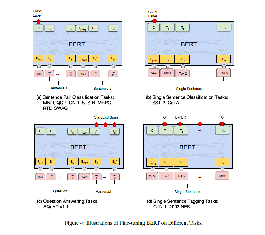
Fine-tuning is straightforward since the self-attention mechanism in the Transformer allows BERT to model many downstream tasks—whether they involve single text or text pairs—by swapping out the appropriate inputs and outputs.
미세 조정은 비교적 간단합니다. 트랜스포머의 self-attention 메커니즘 덕분에 BERT는 단일 텍스트든 문장 쌍이든 관계없이, 적절한 입력과 출력을 교체함으로써 다양한 다운스트림 작업을 쉽게 처리할 수 있습니다.
For applications involving text pairs, a common pattern is to independently encode text pairs before applying bidirectional cross attention, such as Parikh et al. (2016); Seo et al. (2017).
텍스트 쌍을 포함하는 작업에서는 Parikh et al.(2016), Seo et al.(2017)처럼 텍스트 쌍을 독립적으로 인코딩한 후 양방향 크로스 어텐션을 적용하는 방식이 일반적입니다.
BERT instead uses the self-attention mechanism to unify these two stages, as encoding a concatenated text pair with self-attention effectively includes bidirectional cross attention between two sentences.
하지만 BERT는 self-attention 메커니즘을 사용하여 이러한 두 단계를 통합합니다. 하나로 결합된 문장 쌍을 self-attention으로 인코딩하면 자동으로 양방향 크로스 어텐션이 적용되기 때문입니다.
For each task, we simply plug in the task-specific inputs and outputs into BERT and fine-tune all the parameters end-to-end.
각 작업마다 우리는 작업별 입력과 출력을 BERT에 연결한 후 모든 파라미터를 끝까지(end-to-end) 미세 조정합니다.
At the input, sentence A and sentence B from pre-training are analogous to (1) sentence pairs in paraphrasing, (2) hypothesis-premise pairs in entailment, (3) question-passage pairs in question answering, and (4) a degenerate text-? pair in text classification or sequence tagging.
입력 측면에서는 사전 학습에서의 문장 A와 B가 각각 (1) 패러프레이징의 문장 쌍, (2) 엔테일먼트 작업의 가설-전제 쌍, (3) 질의응답의 질문-지문 쌍, (4) 텍스트 분류나 시퀀스 태깅의 텍스트-빈칸 쌍으로 대응됩니다.
At the output, the token representations are fed into an output layer for token-level tasks, such as sequence tagging or question answering, and the [CLS] representation is fed into an output layer for classification, such as entailment or sentiment analysis.
출력 측면에서는 토큰 수준의 작업(예: 시퀀스 태깅, 질의응답)에서는 각 토큰 표현을 출력층에 전달하고, 분류 작업(예: 엔테일먼트, 감정 분석)에서는 [CLS] 벡터를 출력층에 전달합니다.
Compared to pre-training, fine-tuning is relatively inexpensive.
사전 학습에 비해, 미세 조정은 상대적으로 비용이 적게 듭니다.
All of the results in the paper can be replicated in at most 1 hour on a single Cloud TPU, or a few hours on a GPU, starting from the exact same pre-trained model.
논문의 모든 실험 결과는 동일한 사전 학습 모델로부터 Cloud TPU 한 대에서는 1시간 이내, GPU에서는 몇 시간 내에 재현이 가능합니다.
We describe the task-specific details in the corresponding subsections of Section 4.
각 작업별 세부 사항은 4장에 있는 해당 소절에서 설명합니다.
More details can be found in Appendix A.5.
추가적인 자세한 내용은 부록 A.5에서 확인할 수 있습니다.
4 Experiments
4 실험
In this section, we present BERT fine-tuning results on 11 NLP tasks.
이 절에서는 BERT의 미세 조정 결과를 11가지 NLP 작업에 대해 소개합니다.
4.1 GLUE
4.1 GLUE

The General Language Understanding Evaluation (GLUE) benchmark (Wang et al., 2018a) is a collection of diverse natural language understanding tasks.
GLUE (General Language Understanding Evaluation) 벤치마크(Wang et al., 2018a)는 다양한 자연어 이해 과제를 모아 놓은 평가 세트입니다.
Detailed descriptions of GLUE datasets are included in Appendix B.1.
GLUE 데이터셋에 대한 자세한 설명은 부록 B.1에 포함되어 있습니다.
To fine-tune on GLUE, we represent the input sequence (for single sentence or sentence pairs) as described in Section 3, and use the final hidden vector C ∈ RH corresponding to the first input token ([CLS]) as the aggregate representation.
GLUE에 대한 미세 조정 시에는 3장에서 설명한 방법대로 입력 시퀀스를 구성하고, 첫 번째 입력 토큰([CLS])에 해당하는 최종 히든 벡터 C ∈ RH를 전체 시퀀스를 대표하는 벡터로 사용합니다.
The only new parameters introduced during fine-tuning are classification layer weights W ∈ RK×H, where K is the number of labels.
미세 조정 과정에서 새롭게 추가되는 파라미터는 분류 레이어의 가중치 W ∈ RK×H이며, 여기서 K는 레이블의 개수입니다.
We compute a standard classification loss with C and W, i.e., log(softmax(CWT )).
C와 W를 사용하여 표준 분류 손실(로그 소프트맥스)을 계산합니다.
We use a batch size of 32 and fine-tune for 3 epochs over the data for all GLUE tasks.
모든 GLUE 작업에 대해 배치 크기 32로 3 에폭 동안 미세 조정을 수행합니다.
For each task, we selected the best fine-tuning learning rate (among 5e-5, 4e-5, 3e-5, and 2e-5) on the Dev set.
각 작업에 대해 개발 세트(Dev set)에서 가장 좋은 미세 조정 학습률(5e-5, 4e-5, 3e-5, 2e-5 중)을 선택했습니다.
Additionally, for BERTLARGE we found that fine-tuning was sometimes unstable on small datasets, so we ran several random restarts and selected the best model on the Dev set.
또한, BERTLARGE의 경우 소규모 데이터셋에서 미세 조정이 불안정할 때가 있어 여러 번 무작위 초기화(random restart)를 실행하고, 개발 세트에서 가장 좋은 모델을 선택했습니다.
With random restarts, we use the same pre-trained checkpoint but perform different fine-tuning data shuffling and classifier layer initialization.
랜덤 리스타트 시에는 동일한 사전 학습 체크포인트를 사용하지만, 미세 조정 과정에서 데이터 셔플링과 분류 레이어 초기화를 다르게 설정합니다.
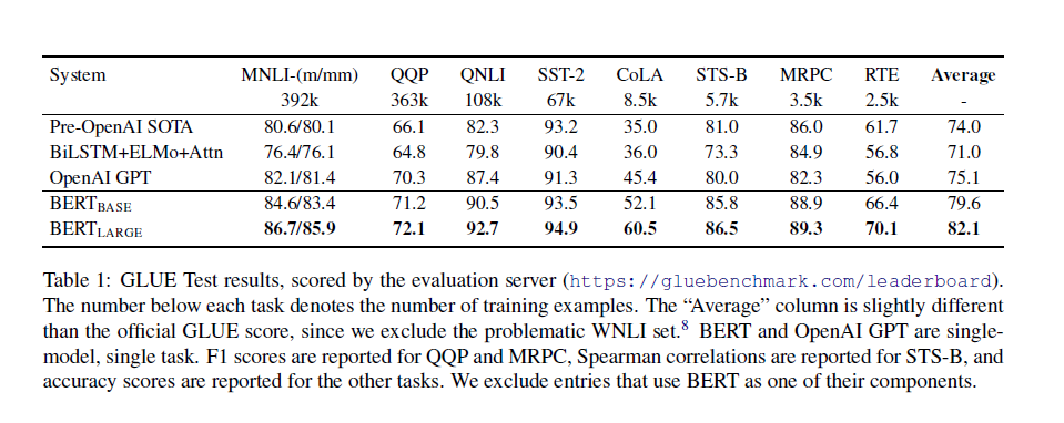
Results are presented in Table 1.
결과는 표 1에 제시되어 있습니다.
Both BERTBASE and BERTLARGE outperform all systems on all tasks by a substantial margin, obtaining 4.5% and 7.0% respective average accuracy improvement over the prior state of the art.
BERTBASE와 BERTLARGE는 모든 과제에서 기존 시스템보다 월등히 뛰어난 성능을 보였으며, 기존 최고 성능 대비 각각 4.5%와 7.0%의 평균 정확도 향상을 달성했습니다.
Note that BERTBASE and OpenAI GPT are nearly identical in terms of model architecture apart from the attention masking.
BERTBASE와 OpenAI GPT는 어텐션 마스킹 방식을 제외하면 모델 아키텍처 측면에서 거의 동일함을 주목할 필요가 있습니다.
For the largest and most widely reported GLUE task, MNLI, BERT obtains a 4.6% absolute accuracy improvement.
GLUE의 가장 큰 과제이자 가장 널리 보고된 작업인 MNLI에서 BERT는 4.6%의 절대 정확도 향상을 기록했습니다.
On the official GLUE leaderboard, BERTLARGE obtains a score of 80.5, compared to OpenAI GPT, which obtains 72.8 as of the date of writing.
공식 GLUE 리더보드에서 BERTLARGE는 80.5점을 기록했으며, OpenAI GPT는 작성 시점 기준 72.8점을 기록했습니다.
We find that BERTLARGE significantly outperforms BERTBASE across all tasks, especially those with very little training data.
모든 과제에서 BERTLARGE가 BERTBASE보다 현저히 뛰어난 성능을 보였으며, 특히 학습 데이터가 적은 과제에서 그 효과가 두드러졌습니다.
The effect of model size is explored more thoroughly in Section 5.2.
모델 크기의 영향에 대한 더 자세한 분석은 5.2절에서 다루고 있습니다.
4.2 SQuAD v1.1
The Stanford Question Answering Dataset (SQuAD v1.1) is a collection of 100k crowdsourced question/answer pairs (Rajpurkar et al., 2016).
스탠포드 질의응답 데이터셋(SQuAD v1.1) 은 크라우드소싱을 통해 수집된 10만 개의 질문/답변 쌍으로 구성되어 있습니다 (Rajpurkar et al., 2016).
Given a question and a passage from Wikipedia containing the answer, the task is to predict the answer text span in the passage.
질문과 답이 포함된 위키피디아 지문이 주어지면, 지문 내에서 정답이 되는 텍스트 구간(span)을 예측하는 것이 과제입니다.
As shown in Figure 1, in the question answering task, we represent the input question and passage as a single packed sequence, with the question using the A embedding and the passage using the B embedding.
그림 1에서 보이는 것처럼, 질의응답 작업에서 입력 질문과 지문은 하나의 시퀀스로 결합되며, 질문에는 A 임베딩, 지문에는 B 임베딩을 적용합니다.
We only introduce a start vector S ∈ RH and an end vector E ∈ RH during fine-tuning.
미세 조정 단계에서 우리는 시작 벡터 S ∈ RH 와 종료 벡터 E ∈ RH 만 새롭게 추가합니다.
The probability of word i being the start of the answer span is computed as a dot product between Ti and S followed by a softmax over all of the words in the paragraph: Pi = e^(S·Ti) / ∑j e^(S·Tj).
단어 i가 정답 시작 위치일 확률은 Ti와 S의 내적(dot product)을 계산한 후, 단락 내 모든 단어에 대해 소프트맥스를 적용하여 구합니다: Pi = e^(S·Ti) / ∑j e^(S·Tj).
The analogous formula is used for the end of the answer span.
정답의 끝 위치를 찾는 것도 동일한 방식의 공식을 사용합니다.
The score of a candidate span from position i to position j is defined as S·Ti + E·Tj, and the maximum scoring span where j ≥ i is used as a prediction.
i 위치에서 j 위치까지의 후보 스팬 점수는 S·Ti + E·Tj 로 정의되며, j ≥ i 조건을 만족하는 최고 점수 스팬이 최종 예측으로 사용됩니다.
The training objective is the sum of the log-likelihoods of the correct start and end positions.
훈련 목표는 정답 시작과 끝 위치의 로그 가능도(log-likelihood) 합을 최대화하는 것입니다.
We fine-tune for 3 epochs with a learning rate of 5e-5 and a batch size of 32.
우리는 학습률 5e-5, 배치 크기 32로 3 에폭 동안 미세 조정합니다.
Table 2 shows top leaderboard entries as well as results from top published systems (Seo et al., 2017; Clark and Gardner, 2018; Peters et al., 2018a; Hu et al., 2018).
표 2에는 상위 리더보드 결과와 주요 논문 시스템(Seo et al., 2017; Clark and Gardner, 2018; Peters et al., 2018a; Hu et al., 2018)의 성능이 비교되어 있습니다.
The top results from the SQuAD leaderboard do not have up-to-date public system descriptions available, and are allowed to use any public data when training their systems.
SQuAD 리더보드 상위 모델들은 최신 공개 시스템 설명이 제공되지 않으며, 학습 시 공개된 모든 데이터를 사용할 수 있습니다.
We therefore use modest data augmentation in our system by first fine-tuning on TriviaQA (Joshi et al., 2017) before fine-tuning on SQuAD.
따라서 우리는 SQuAD에 미세 조정하기 전에 TriviaQA (Joshi et al., 2017)로 선행 미세 조정을 진행하는 방식으로 소폭 데이터 증강을 활용했습니다.
Our best performing system outperforms the top leaderboard system by +1.5 F1 in ensembling and +1.3 F1 as a single system.
우리의 최상위 성능 시스템은 앙상블 기준으로 리더보드 최고 시스템보다 +1.5 F1, 단일 모델 기준으로 +1.3 F1 더 높은 성능을 보였습니다.
In fact, our single BERT model outperforms the top ensemble system in terms of F1 score.
실제로 우리의 단일 BERT 모델이 F1 점수 면에서 기존 최고 앙상블 시스템보다 뛰어났습니다.
Without TriviaQA fine-tuning data, we only lose 0.1–0.4 F1, still outperforming all existing systems by a wide margin.
TriviaQA로 사전 미세 조정 없이도 F1 점수가 0.1~0.4 정도만 감소했으며, 여전히 기존 모든 시스템을 큰 차이로 능가했습니다.
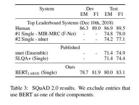
4.3 SQuAD v2.0
The SQuAD 2.0 task extends the SQuAD 1.1 problem definition by allowing for the possibility that no short answer exists in the provided paragraph, making the problem more realistic.
SQuAD 2.0 작업은 SQuAD 1.1 문제 정의를 확장하여, 주어진 지문에 짧은 정답이 존재하지 않을 가능성을 포함함으로써 문제를 더욱 현실적으로 만듭니다.
We use a simple approach to extend the SQuAD v1.1 BERT model for this task.
이 작업을 위해 우리는 SQuAD v1.1용 BERT 모델을 단순히 확장하는 방법을 사용했습니다.
We treat questions that do not have an answer as having an answer span with start and end at the [CLS] token.
답이 존재하지 않는 질문은 시작과 끝 위치가 [CLS] 토큰인 답변 스팬으로 간주합니다.
The probability space for the start and end answer span positions is extended to include the position of the [CLS] token.
정답 스팬의 시작 및 끝 위치를 나타내는 확률 공간은 [CLS] 토큰 위치를 포함하도록 확장됩니다.
For prediction, we compare the score of the no-answer span: snull = S·C + E·C to the score of the best non-null span ŝi,j = max_{j≥i} (S·Ti + E·Tj).
예측 시, 정답 없음(no-answer) 스팬의 점수 snull = S·C + E·C와 최고 점수를 갖는 실제 스팬 ŝi,j = max_{j≥i} (S·Ti + E·Tj) 를 비교합니다.
We predict a non-null answer when ŝi,j > snull + ϴ, where the threshold ϴ is selected on the dev set to maximize F1.
ŝi,j > snull + ϴ 조건을 만족하면 답변이 있다고 예측하며, 여기서 임계값(ϴ) 는 개발 세트에서 F1 점수를 극대화하도록 선택됩니다.
We did not use TriviaQA data for this model.
이 모델에는 TriviaQA 데이터를 사용하지 않았습니다.
We fine-tuned for 2 epochs with a learning rate of 5e-5 and a batch size of 48.
우리는 학습률 5e-5, 배치 크기 48로 2 에폭 동안 미세 조정을 수행했습니다.
The results compared to prior leaderboard entries and top published work (Sun et al., 2018; Wang et al., 2018b) are shown in Table 3, excluding systems that use BERT as one of their components.
이전 리더보드 결과 및 주요 논문 시스템(Sun et al., 2018; Wang et al., 2018b)과의 비교 결과는 표 3에 나타나 있으며, BERT를 일부로 사용하는 시스템은 제외했습니다.
We observe a +5.1 F1 improvement over the previous best system.
우리는 이전 최고 성능 시스템 대비 +5.1 F1 점수 향상을 확인했습니다.
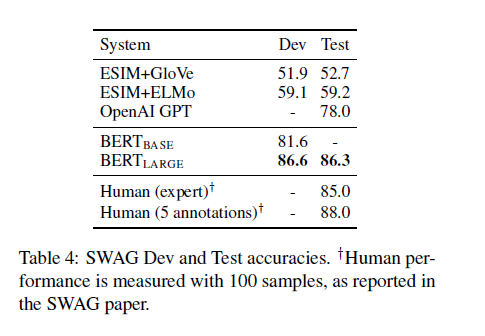
4.4 SWAG
The Situations With Adversarial Generations (SWAG) dataset contains 113k sentence-pair completion examples that evaluate grounded commonsense inference (Zellers et al., 2018).
SWAG (Situations With Adversarial Generations) 데이터셋은 113,000개의 문장 쌍 완성 예제를 포함하고 있으며, 상황 기반 상식 추론 능력을 평가합니다 (Zellers et al., 2018).
Given a sentence, the task is to choose the most plausible continuation among four choices.
하나의 문장이 주어지면, 네 가지 선택지 중 가장 그럴듯한 문장 이어쓰기를 선택하는 것이 과제입니다.
When fine-tuning on the SWAG dataset, we construct four input sequences, each containing the concatenation of the given sentence (sentence A) and a possible continuation (sentence B).
SWAG 데이터셋에서 미세 조정 시, 주어진 문장(문장 A)과 가능한 후속 문장(문장 B)을 결합하여 네 개의 입력 시퀀스를 만듭니다.
The only task-specific parameters introduced is a vector whose dot product with the [CLS] token representation C denotes a score for each choice which is normalized with a softmax layer.
작업별로 새롭게 추가되는 파라미터는 [CLS] 벡터 C 와 내적을 계산해 각 선택지의 점수를 구하고, 이 점수를 소프트맥스 레이어로 정규화하는 하나의 벡터 뿐입니다.
We fine-tune the model for 3 epochs with a learning rate of 2e-5 and a batch size of 16.
우리는 학습률 2e-5, 배치 크기 16으로 3 에폭 동안 모델을 미세 조정했습니다.
Results are presented in Table 4.
결과는 표 4에 제시되어 있습니다.
BERTLARGE outperforms the authors’ baseline ESIM+ELMo system by +27.1% and OpenAI GPT by 8.3%.
BERTLARGE는 저자들이 제안한 ESIM+ELMo 베이스라인보다 27.1%, OpenAI GPT보다 8.3% 높은 성능을 기록했습니다.
5 Ablation Studies
5 절제 실험(Ablation Studies)
In this section, we perform ablation experiments over a number of facets of BERT in order to better understand their relative importance.
이 절에서는 BERT의 여러 구성 요소에 대한 절제(ablation) 실험을 수행하여 각 요소의 상대적인 중요성을 이해합니다.
Additional ablation studies can be found in Appendix C.
추가적인 절제 실험 결과는 부록 C에서 확인할 수 있습니다.
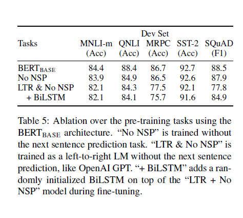
5.1 Effect of Pre-training Tasks
5.1 사전 학습 작업의 영향
We demonstrate the importance of the deep bidirectionality of BERT by evaluating two pretraining objectives using exactly the same pretraining data, fine-tuning scheme, and hyperparameters as BERTBASE:
BERT의 깊은 양방향성의 중요성을 보여주기 위해, BERTBASE와 동일한 사전 학습 데이터, 미세 조정 방식, 하이퍼파라미터를 사용해 두 가지 사전 학습 목표를 평가했습니다.
No NSP: A bidirectional model which is trained using the “masked LM” (MLM) but without the “next sentence prediction” (NSP) task.
No NSP: NSP(다음 문장 예측) 없이 MLM(마스크드 언어 모델) 만으로 훈련한 양방향 모델입니다.
LTR & No NSP: A left-context-only model which is trained using a standard Left-to-Right (LTR) LM, rather than an MLM.
LTR & No NSP: MLM 대신 표준적인 왼쪽-오른쪽(LTR) 언어 모델로 훈련된 좌측 문맥 전용 모델입니다.
The left-only constraint was also applied at fine-tuning, because removing it introduced a pre-train/fine-tune mismatch that degraded downstream performance.
좌측 방향 제약은 미세 조정 단계에서도 유지했는데, 이를 제거하면 사전 학습과 미세 조정 간 불일치가 발생해 성능 저하로 이어졌기 때문입니다.
Additionally, this model was pre-trained without the NSP task.
이 모델 역시 NSP 없이 사전 학습되었습니다.
This is directly comparable to OpenAI GPT, but using our larger training dataset, our input representation, and our fine-tuning scheme.
이 모델은 OpenAI GPT와 직접 비교할 수 있지만, 우리는 더 큰 훈련 데이터셋, BERT의 입력 표현 방식, 그리고 우리의 미세 조정 방식을 사용했습니다.
We first examine the impact brought by the NSP task.
우리는 먼저 NSP 작업이 미치는 영향을 살펴보았습니다.
In Table 5, we show that removing NSP hurts performance significantly on QNLI, MNLI, and SQuAD 1.1.
표 5에서 보듯이, NSP를 제거하면 QNLI, MNLI, SQuAD 1.1 과제에서 성능이 크게 저하됩니다.
Next, we evaluate the impact of training bidirectional representations by comparing “No NSP” to “LTR & No NSP.”
다음으로, 양방향 표현 학습의 중요성을 확인하기 위해 "No NSP" 모델과 "LTR & No NSP" 모델을 비교했습니다.
The LTR model performs worse than the MLM model on all tasks, with large drops on MRPC and SQuAD.
LTR 모델은 모든 작업에서 MLM 모델보다 성능이 낮았으며, 특히 MRPC와 SQuAD에서 큰 성능 저하가 나타났습니다.
For SQuAD it is intuitively clear that a LTR model will perform poorly at token predictions, since the token-level hidden states have no right-side context.
SQuAD의 경우 LTR 모델은 오른쪽 문맥 정보가 없기 때문에 토큰 예측에서 성능이 떨어질 수밖에 없다는 점은 직관적으로 이해할 수 있습니다.
In order to make a good faith attempt at strengthening the LTR system, we added a randomly initialized BiLSTM on top.
LTR 시스템을 개선하기 위해 랜덤 초기화된 BiLSTM 층을 추가해 보았습니다.
This does significantly improve results on SQuAD, but the results are still far worse than those of the pre-trained bidirectional models.
이로 인해 SQuAD 성능은 어느 정도 개선되었으나, 여전히 사전 학습된 양방향 모델에 비해 크게 부족했습니다.
The BiLSTM hurts performance on the GLUE tasks.
게다가 BiLSTM 추가는 GLUE 작업의 성능을 오히려 저하시켰습니다.
We recognize that it would also be possible to train separate LTR and RTL models and represent each token as the concatenation of the two models, as ELMo does.
ELMo처럼 LTR과 RTL 모델을 따로 학습하고 두 모델의 출력을 결합하여 각 토큰을 표현하는 방식도 가능하다는 점을 인지하고 있습니다.
However: (a) this is twice as expensive as a single bidirectional model;
하지만 이 방식은 (a) 양방향 모델에 비해 2배의 연산 비용이 소요되며,
(b) this is non-intuitive for tasks like QA, since the RTL model would not be able to condition the answer on the question;
(b) 질의응답(QA) 과 같은 작업에서는 RTL 모델이 질문에 조건을 걸지 못해 직관적이지 않고,
(c) this is strictly less powerful than a deep bidirectional model, since it can use both left and right context at every layer.
(c) 모든 레이어에서 좌우 문맥을 동시에 활용할 수 있는 깊은 양방향 모델에 비해 표현력이 떨어진다는 한계가 있습니다.
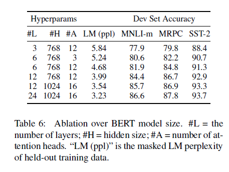
5.2 Effect of Model Size
5.2 모델 크기의 영향
In this section, we explore the effect of model size on fine-tuning task accuracy.
이 절에서는 모델 크기가 미세 조정(fine-tuning) 작업의 정확도에 미치는 영향을 살펴봅니다.
We trained a number of BERT models with a differing number of layers, hidden units, and attention heads, while otherwise using the same hyperparameters and training procedure as described previously.
우리는 레이어 수, 히든 유닛 수, 어텐션 헤드 수가 다른 여러 BERT 모델을 훈련했으며, 그 외의 하이퍼파라미터와 학습 절차는 앞서 설명한 내용과 동일하게 유지했습니다.
Results on selected GLUE tasks are shown in Table 6.
선택된 GLUE 작업에 대한 결과는 표 6에 제시되어 있습니다.

In this table, we report the average Dev Set accuracy from 5 random restarts of fine-tuning.
이 표에는 5번의 무작위 초기화를 통한 미세 조정 결과의 개발 세트 평균 정확도가 보고되어 있습니다.
We can see that larger models lead to a strict accuracy improvement across all four datasets, even for MRPC which only has 3,600 labeled training examples, and is substantially different from the pre-training tasks.
모델이 클수록 모든 4개 데이터셋에서 일관된 정확도 향상이 나타났으며, 심지어 사전 학습 작업과 성격이 매우 다르고 라벨이 3,600개에 불과한 MRPC 데이터셋에서도 향상이 있었습니다.
It is also perhaps surprising that we are able to achieve such significant improvements on top of models which are already quite large relative to the existing literature.
이미 기존 연구에 비해 충분히 큰 모델 위에서도 이렇게 큰 성능 향상을 달성할 수 있다는 점은 놀라운 결과입니다.
For example, the largest Transformer explored in Vaswani et al. (2017) is (L=6, H=1024, A=16) with 100M parameters for the encoder, and the largest Transformer we have found in the literature is (L=64, H=512, A=2) with 235M parameters (Al-Rfou et al., 2018).
예를 들어, Vaswani et al.(2017)에서 다룬 가장 큰 트랜스포머는 (L=6, H=1024, A=16) 로 1억 개의 파라미터를 갖는 인코더였고, 우리가 찾은 문헌상 가장 큰 트랜스포머는 (L=64, H=512, A=2) 으로 2억 3,500만 개의 파라미터를 갖는 모델(Al-Rfou et al., 2018)이었습니다.
By contrast, BERTBASE contains 110M parameters and BERTLARGE contains 340M parameters.
이에 비해, BERTBASE는 1억 1천만 개, BERTLARGE는 3억 4천만 개의 파라미터를 가집니다.
It has long been known that increasing the model size will lead to continual improvements on large-scale tasks such as machine translation and language modeling, which is demonstrated by the LM perplexity of held-out training data shown in Table 6.
모델 크기를 키우면 기계 번역과 언어 모델링 같은 대규모 작업에서 꾸준한 성능 향상이 나타난다는 것은 잘 알려진 사실이며, 이는 표 6의 언어 모델 퍼플렉서티(LM perplexity) 수치로도 확인됩니다.

However, we believe that this is the first work to demonstrate convincingly that scaling to extreme model sizes also leads to large improvements on very small scale tasks, provided that the model has been sufficiently pre-trained.
하지만, 충분히 사전 학습된 모델이라면 아주 작은 규모의 작업에서도 모델 크기를 극단적으로 키우는 것이 큰 성능 향상을 가져올 수 있음을 명확히 입증한 것은 본 연구가 처음이라고 생각합니다.
Peters et al. (2018b) presented mixed results on the downstream task impact of increasing the pre-trained bi-LM size from two to four layers and Melamud et al. (2016) mentioned in passing that increasing hidden dimension size from 200 to 600 helped, but increasing further to 1,000 did not bring further improvements.
Peters et al.(2018b)는 사전 학습된 양방향 언어 모델(bi-LM) 의 레이어를 2층에서 4층으로 늘렸을 때 다운스트림 작업에서 혼재된 결과를 보고했으며, Melamud et al.(2016) 도 히든 차원을 200에서 600으로 키우면 도움이 되었지만, 1,000으로 더 늘리는 것은 추가 효과가 없다고 언급한 바 있습니다.
Both of these prior works used a feature-based approach — we hypothesize that when the model is fine-tuned directly on the downstream tasks and uses only a very small number of randomly initialized additional parameters, the task-specific models can benefit from the larger, more expressive pre-trained representations even when downstream task data is very small.
이러한 기존 연구들은 모두 feature-based 방식을 사용했으며, 우리는 모델이 다운스트림 작업에 직접 미세 조정되고 소수의 무작위 초기화된 추가 파라미터만 사용할 경우, 다운스트림 작업의 데이터가 매우 적더라도 더 크고 표현력이 뛰어난 사전 학습 표현으로부터 큰 이득을 얻을 수 있다는 가설을 제시합니다.
5.3 Feature-based Approach with BERT
5.3 BERT의 Feature-based 접근법
All of the BERT results presented so far have used the fine-tuning approach, where a simple classification layer is added to the pre-trained model, and all parameters are jointly fine-tuned on a downstream task.
지금까지 제시된 BERT의 모든 결과는 사전 학습된 모델 위에 단순한 분류 레이어를 추가하고, 모든 파라미터를 다운스트림 작업에 맞게 함께 미세 조정(fine-tuning) 하는 방식을 사용했습니다.
However, the feature-based approach, where fixed features are extracted from the pre-trained model, has certain advantages.
하지만 feature-based 접근법, 즉 사전 학습된 모델에서 고정된 특징(feature) 만 추출해서 사용하는 방식도 몇 가지 장점이 있습니다.
First, not all tasks can be easily represented by a Transformer encoder architecture, and therefore require a task-specific model architecture to be added.
첫째, 모든 작업이 트랜스포머 인코더 아키텍처로 쉽게 표현되지 않기 때문에, 작업에 특화된 모델 아키텍처를 추가로 설계해야 할 수도 있습니다.
Second, there are major computational benefits to pre-compute an expensive representation of the training data once and then run many experiments with cheaper models on top of this representation.
둘째, 계산 비용이 큰 표현을 한 번만 사전 계산 해두고, 이 위에 가벼운 모델로 여러 실험을 반복 실행할 수 있다는 계산 효율상의 이점이 있습니다.
In this section, we compare the two approaches by applying BERT to the CoNLL-2003 Named Entity Recognition (NER) task (Tjong Kim Sang and De Meulder, 2003).
이 절에서는 CoNLL-2003 개체명 인식(NER) 작업(Tjong Kim Sang & De Meulder, 2003)에 BERT를 적용해 두 가지 접근법을 비교했습니다.
In the input to BERT, we use a case-preserving WordPiece model, and we include the maximal document context provided by the data.
BERT 입력 시에는 대소문자를 유지하는 WordPiece 모델을 사용하며, 데이터에서 제공되는 최대한의 문서 컨텍스트를 포함시켰습니다.
Following standard practice, we formulate this as a tagging task but do not use a CRF layer in the output.
표준적인 방식에 따라 이 작업을 태깅 작업으로 정의했으며, 출력에는 CRF 레이어를 사용하지 않았습니다.
We use the representation of the first sub-token as the input to the token-level classifier over the NER label set.
각 토큰의 첫 번째 서브토큰의 표현을 NER 레이블 분류기의 입력으로 사용했습니다.
To ablate the fine-tuning approach, we apply the feature-based approach by extracting the activations from one or more layers without fine-tuning any parameters of BERT.
미세 조정 접근법의 영향을 분리 분석하기 위해, BERT의 파라미터를 미세 조정하지 않고, 한 층 또는 여러 층의 활성화 값(activation) 을 추출하는 feature-based 방식을 적용했습니다.
These contextual embeddings are used as input to a randomly initialized two-layer 768-dimensional BiLSTM before the classification layer.
이렇게 추출된 문맥 임베딩은 무작위 초기화된 2층 768차원 BiLSTM 의 입력으로 사용한 후, 분류층에 전달했습니다.
Results are presented in Table 7.
결과는 표 7에 나와 있습니다.
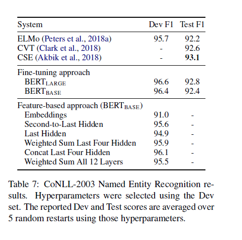
BERTLARGE performs competitively with state-of-the-art methods.
BERTLARGE는 최첨단 방법들과 비교해도 경쟁력 있는 성능을 보였습니다.
The best performing method concatenates the token representations from the top four hidden layers of the pre-trained Transformer, which is only 0.3 F1 behind fine-tuning the entire model.
가장 성능이 뛰어났던 방식은 사전 학습된 트랜스포머의 상위 4개 히든 레이어의 토큰 표현을 결합(concatenate) 한 방법이었으며, 전체 모델을 미세 조정하는 것보다 F1 점수가 단 0.3 낮았습니다.
This demonstrates that BERT is effective for both fine-tuning and feature-based approaches.
이는 BERT가 fine-tuning 방식과 feature-based 방식 모두에 효과적임을 보여줍니다.
6 Conclusion
6 결론
Recent empirical improvements due to transfer learning with language models have demonstrated that rich, unsupervised pre-training is an integral part of many language understanding systems.
최근 언어 모델 기반 전이 학습(transfer learning) 에서의 경험적 성과는, 풍부한 비지도 사전 학습이 많은 언어 이해 시스템의 핵심 요소라는 점을 입증했습니다.
In particular, these results enable even low-resource tasks to benefit from deep unidirectional architectures.
특히, 이러한 결과는 자원이 적은 작업(low-resource tasks) 조차도 깊은 단방향 아키텍처의 혜택을 볼 수 있음을 보여줍니다.
Our major contribution is further generalizing these findings to deep bidirectional architectures, allowing the same pre-trained model to successfully tackle a broad set of NLP tasks.
우리 연구의 가장 큰 기여는 이러한 발견을 깊은 양방향 아키텍처로 일반화했으며, 이를 통해 하나의 사전 학습 모델로 광범위한 NLP 작업을 성공적으로 처리할 수 있게 한 점입니다.