W4

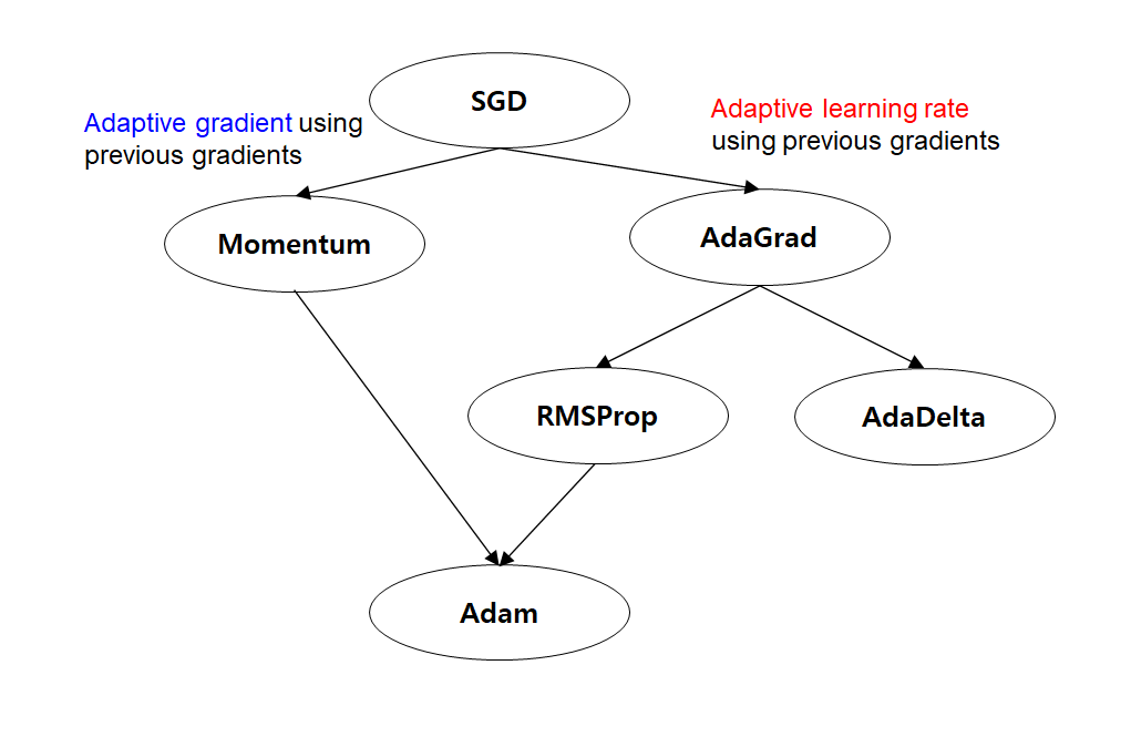
• Momentum의 장점
• • 만약 연속되는 gradient step이 다른 방향이라면, 그 방향을 disagree함. 만약 연속되는 gradient step이 비슷한 방향이라면, 그 방향으로 더 빠르게 수렴함
• • 관성을 활용하여 이전의 gradient 정보를 사용해 현재의 gradient를 업데이트 함으로써, 최적화 과정에서 더 빠른 수렴을 이끌어냄
• • Local minima에 빠지지 않고 Global minima로 더 안정적으로 수렴할 수 있음
• • 최적화 과정에서 높은 속도로 수렴하여 빠른 학습 속도를 가질 수 있음
• RMSProp의 장점
• • Adagrad의 문제인 변화량이 클수록 learing rate가 작아져 조기 종료되는 문제를 해결하기 위해 learning rate의 크기를 비율로 조정할 수 있음
• • 각각의 parameter마다 다른 learning rate를 가질 수 있어, 더 동적인 학습 속도를 제공함
• • 기존의 AdaGrad에서 누적된 gradient 제곱 값을 지수 이동 평균을 사용해 더 간결한 parameter 업데이트를 수행함
• • 안정적인 학습 속도를 제공하면서, Local minima에 빠지는 문제를 완화할 수 있음

MLP1 = torch.nn.Linear(3,4)     #nn.Linear(input_dim, output_dim)
print(f'MLP1.weight {MLP1.weight}, MLP1.bias {MLP1.bias}')
MLP2 = torch.nn.Linear(4,1)
print(f'\n MLP2.weight {MLP2.weight}, MLP2.bias {MLP2.bias}')

x = torch.tensor([1., 0., 1.]) # input data
target = torch.tensor(0.5) # target data
optim = torch.optim.SGD([MLP1.weight, MLP1.bias, MLP2.weight, MLP2.bias], lr=0.1) # parameter 학습에 Stochastic gradient descent를 사용
loss_func = torch.nn.MSELoss() # Mean Squared Error function을 사용

for i in range(5):
  y = MLP1(x)
  y = torch.nn.functional.sigmoid(y)
  y = MLP2(y)
  y = torch.nn.functional.sigmoid(y)
  loss = loss_func(y, target)
  # pytorch automaticaaly calculates the gradient and applies EBP(Error Back Propagation)
  optim.zero_grad()     # zero_grad() function is making the gradient zero..this time is for initialization
  loss.backward()       # pytorch automatically calculates the gradient
  optim.step()          # update the weights
  print(loss)

• 저번주에 했던 내용

# Momentum is caring about the past gradient and uses the past gradient as well!
# momentum can be assigned in the SGD function torch implemented
MLP1 = torch.nn.Linear(3, 1)
optimizer = torch.optim.SGD(MLP1.parameters(), lr= 0.001, momentum=0.9) # Stochastic Gradient Descent에 momentum을 옵션으로 줌

• Optimization method: momentum

# RMSProp adjusts the learning rate for each weight, if the gradient was large at the past history, learning rate becomes smallar -> 조기 종료되는 문제를 해결할 수 있음
# RMSProp 
optimizer = torch.optim.RMSprop(MLP1.parameters(), lr =0.001) #늘 쓰던 SGD가 아닌, RMSProp을 사용하여 최적화

• Optimization method: RMSProp

# Adam is somewhat having characteristics of both the momentum and RMSProp as you can figure out in the figure
optimizer = torch.optim.Adam(MLP1.parameters(), lr = 0.001) # momentum과 RMSProp의 장점을 살린 Adam optimizer를 사용

• Optimization method: Adam/ 이번주는 Adam optimizer를 사용

class Titanic_layer(torch.nn.Module):
  def __init__(self):
    super(Titanic_layer, self).__init__()
    ## define your own layers! 
    self.MLP1 = torch.nn.Linear(10, 32) #(input_dim, output_dim)
    self.MLP2 = torch.nn.Linear(32, 64)
    self.MLP3 = torch.nn.Linear(64, 32)
    self.MLP4 = torch.nn.Linear(32, 16)
    self.MLP5 = torch.nn.Linear(16, 4)
    self.MLP6 = torch.nn.Linear(4, 1)

  def forward(self, x):
    # define the forward function
    y = self.MLP1(x)
    y = torch.nn.functional.relu(y) # we will use relu as our activation function. relu has advantage when layers go deeper!
    y = self.MLP2(y)
    y = torch.nn.functional.relu(y)
    y = self.MLP3(y)
    y = torch.nn.functional.relu(y)
    y = self.MLP4(y)
    y = torch.nn.functional.relu(y)
    y = self.MLP5(y)
    y = torch.nn.functional.relu(y)
    y = self.MLP6(y)
    y = torch.nn.functional.sigmoid(y) #last element should be with 0~1, therefore, we can't use relu
    return y

• relu는 layers가 깊어질 때 효과가 좋음
• 마지막 값은 0 ~ 1 값을 가져야하기 때문에 sigmoid로

epochs = 1000       # please write your own epoch higher than 500
model = Titanic_layer()
loss_func = torch.nn.BCELoss() # loss function으로 Binary Cross Entropy loss function을 사용
optim = torch.optim.Adam(model.parameters(), lr = 0.001) # optimizer로 Adam을 사용
train_total_acc = []
test_total_acc = []
for epoch in range(1, epochs+1):
  train_acc = 0
  train_total = 0
  test_acc = 0
  test_total = 0
  for i, data in enumerate(train_dataloader):
    x, target = data
    model.train() # this code indicates that model is in training mode
    y = model(x)
    loss = loss_func(y, target)
    real_y = (y>=0.5).float()
    train_acc += (real_y == target).float().sum()
    train_total += target.shape[0]
    optim.zero_grad()
    loss.backward()
    optim.step()
  for i, data in enumerate(test_dataloader):
    x, target = data
    model.eval() # this code indicates that model is in evaluation mode
    with torch.no_grad():
      y = model(x)
      loss = loss_func(y, target)
      real_y = (y>=0.5).float()
      test_acc += (real_y == target).float().sum()
      test_total += target.shape[0]
  train_total_acc.append(train_acc/train_total)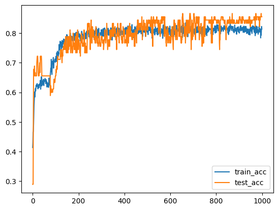
  test_total_acc.append(test_acc/test_total)

• 이렇게 하면 epochs가 늘어날 수록, train_acc는 증가하지만, test_acc는 오히려 감소함 -> overfitting

dropout = torch.nn.Dropout(p=0.7) # p (float) – probability of an element to be zeroed. Default: 0.5
dropout(input)

• 이런 식으로 random하게 일정 비율의 weights를 0으로 바꿔줌 -> 0이 된 weights는 training에 사용되지 않음 -> dropout
  
• dropout을 함으로써, random한 뉴런을 0으로 만듦 -> 모델이 학습 데이터에 대해 과적합되는 것을 완화하고, 더 일반화된 모델을 학습할 수 있게 됨

class Titanic_layer(torch.nn.Module):
  def __init__(self):
    super(Titanic_layer, self).__init__()
    ## define your own layers! 
    self.MLP1 = torch.nn.Linear(10, 32)
    self.MLP2 = torch.nn.Linear(32, 64)
    self.MLP3 = torch.nn.Linear(64, 32)
    self.MLP4 = torch.nn.Linear(32, 16)
    self.MLP5 = torch.nn.Linear(16, 4)
    self.MLP6 = torch.nn.Linear(4, 1)
    # write down the dropout as you want
    self.drop1 = torch.nn.Dropout(p=0.5)
    self.drop2 = torch.nn.Dropout(p=0.7)

  def forward(self, x):
    # define the forward function
    # use the dropout function after the activation function
    y = self.MLP1(x)
    y = torch.nn.functional.relu(y) # we will use relu as our activation function. relu has advantage when layers go deeper!
    y = self.drop1(y)

    y = self.MLP2(y)
    y = torch.nn.functional.relu(y)
    y = self.drop2(y)

    y = self.MLP3(y)
    y = torch.nn.functional.relu(y)
    y = self.drop1(y)

    y = self.MLP4(y)
    y = torch.nn.functional.relu(y)
    y = self.drop2(y)

    y = self.MLP5(y)
    y = torch.nn.functional.relu(y)

    y = self.MLP6(y)
    y = torch.nn.functional.sigmoid(y) #last element should be with 0~1, therefore, we can't use relu
    return y

• dropout을 추가한 Titanic_layer (classification) 정의

epoches = 1000       # please write your own number of epoch same us above 
model = Titanic_layer()
loss_func = torch.nn.BCELoss()
optim = torch.optim.Adam(model.parameters(), lr = 0.001)
train_total_acc = []
test_total_acc = []
for epoch in range(1, epoches+1):
  train_acc = 0
  train_total = 0
  test_acc = 0
  test_total = 0
  for i, data in enumerate(train_dataloader):
    x, target = data
    model.train() # this code indicates that model is in training mode
    y = model(x)
    loss = loss_func(y, target)
    real_y = (y>=0.5).float()
    train_acc += (real_y == target).float().sum()
    train_total += target.shape[0]
    optim.zero_grad()
    loss.backward()
    optim.step()
  for i, data in enumerate(test_dataloader):
    x, target = data
    model.eval() # this code indicates that model is in evaluation mode
    with torch.no_grad():
      y = model(x)
      loss = loss_func(y, target)
      real_y = (y>=0.5).float()
      test_acc += (real_y == target).float().sum()
      test_total += target.shape[0]
  train_total_acc.append(train_acc/train_total)
  test_total_acc.append(test_acc/test_total)

• dropout을 추가한 Titanic_layer를 training & testing
  

Hyper-parameter tuning: Split data into Train, Validation, Test dataset

• hyper-parameters란 learning rate, Batch size, # of Epochs, # of Units in a Layer, Dropout Rate 등임
• models의 성능 향상을 위해, model의 hyper-parameters를 튜닝할 수 있음
• validation dataset은 hyper-parameters tuning에 사용됨. (not test dataset)
• train dataset을 train, validation으로 나눠야함
  

Hyper-parameters tuning: cross-validated grid-search

• 데이터를 세 개의 set (train, validation, test)으로 나눌 때, 샘플링 편향의 위험이 있음
• 이러한 샘플링 편향의 위험을 완화하고, 제한된 데이터를 효율적으로 활용하기 위해 Cross-Validation을 사용함
  

from sklearn.model_selection import KFold
dataset = np.array(train.index)
kf = KFold(n_splits=3, shuffle=True, random_state=42)
for train_idx, val_idx in kf.split(dataset):
  display(train.loc[dataset[val_idx]].head(3))
# cross-validation -> train dataset과 test dataset을 나누고, train dataset을 3부분으로 나눔. 0, 1, 2라고 할 때, 첫번째는 1, 2를 이용해 train하고 0으로 validation, 두번째는 0, 2를 이용해 train하고 1로 validation.. 을 반복한 후 3개의 평균을 구함

Cross-validated grid-search

1. tuning하고싶은 hyper-parameters를 선택

print(net.get_params().keys())

2. 각 hyper-parameters에 대한 cadidate values를 설정

params = {'optimizer':[torch.optim.Adam,torch.optim.RMSprop],
          'lr':[0.001, 0.005, 0.01]}

3. grid search method를 사용하여 model에 적용

from sklearn.model_selection import GridSearchCV
gs = GridSearchCV(estimator=net, 
                  param_grid=params,
                  scoring=my_accuracy, 
                  cv=3, 
                  verbose=0)

gs.fit(X, y) # 모델을 학습시킴

4. model의 best set of hyper-parameters를 반환받음

print(f'Accuracy: {gs.best_score_ * 100 :.2f}%')
print(gs.best_params_)

• grid search는 머신 러닝 모델의 hyper parameters를 최적화하는 기술 -> 모델의 성능을 최적화하기 위해 여러가지 hyper parameters 조합을 시도함
• 미리 정의된 hyper parameters의 가능한 조합들을 그리드 형태로 지정하고, 이들 조합에 대해 Cross validation을 수행하여 각 조합의 모델 성능을 평가함
• 최적의 hyper parameters 조합을 찾아내고, 이를 사용하여 머신 러닝 모델을 훈련시킬 수 있음
• grid search는 모델의 성능을 최적화하는데 유용하며, Cross validation과 함께 사용되어 모델의 성능 평가와 hyper parameters 최적화를 한 번에 수행할 수 있음

# You can refer the above plot of accuray to decide the range of epochs
params = {'max_epochs': [600, 300, 200],  
          'lr':[0.001, 0.005, 0.01]} # optimize한 hyper parameter를 찾기 위함. epochs와 learning rate를 찾을거임

gs = GridSearchCV(estimator=net, 
                  param_grid=params,
                  scoring=my_accuracy, 
                  cv=3, 
                  verbose=0)

gs.fit(X, y) # 모델을 학습시킴

print(f'Accuracy: {gs.best_score_ * 100 :.2f}%')
print(gs.best_params_)

• learning rate는 candidate set 중에서 0.001이, max_epochs는 600이 출력됨

grid search를 통해 찾은 hyper parameters로 K-fold Cross-validation 적용

f = KFold(n_splits=3, shuffle=True, random_state=42)


df = pd.read_csv(io.BytesIO(uploaded['train_preprocessed.csv']))
X_df = df.drop(['Survived'], axis=1)
y_df = df['Survived']

X_df = torch.FloatTensor(X_df.to_numpy())
y_df= torch.FloatTensor(y_df.to_numpy()).reshape(-1, 1)

optimal_epochs = 600  # optimal_epochs and lr -> 위에서 cross-validated grid search method로 찾음
optimal_lr = 0.001

kf = KFold(n_splits=5, shuffle=True, random_state=42)
for fold, (train_idx,val_idx) in enumerate(kf.split(range(len(df)))):

  print('Fold {}'.format(fold + 1))
  train_X = X_df[train_idx]
  train_Y = y_df[train_idx]
  valid_X = X_df[val_idx]
  valid_Y = y_df[val_idx]
  train_dataset = TensorDataset(train_X, train_Y)
  valid_dataset = TensorDataset(valid_X, valid_Y)
  train_dataloader = DataLoader(train_dataset, batch_size=64)
  test_dataloader = DataLoader(valid_dataset, batch_size=64)

  model = Titanic_layer()
  loss_func = torch.nn.BCELoss()
  optim = torch.optim.Adam(model.parameters(), lr = optimal_lr)

  history = {'train_acc':[],'test_acc':[]}
    
  train_acc_lst = []
  test_acc_lst = []

  for epoch in range(1, optimal_epochs+1):
    train_acc = 0
    train_total = 0
    test_acc = 0
    test_total = 0

    for i, data in enumerate(train_dataloader):
      x, target = data
      model.train() # this code indicates that model is in training mode
      y = model(x)
      loss = loss_func(y, target)
      real_y = (y>=0.5).float()
      train_acc += (real_y == target).float().sum()
      train_total += target.shape[0]
      optim.zero_grad()
      loss.backward()
      optim.step()

    for i, data in enumerate(test_dataloader):
      x, target = data
      model.eval() # this code indicates that model is in evaluation mode
      with torch.no_grad():
        y = model(x)
        loss = loss_func(y, target)
        real_y = (y>=0.5).float()
        test_acc += (real_y == target).float().sum()
        test_total += target.shape[0]

    train_acc_lst.append(train_acc/train_total)
    test_acc_lst.append(test_acc/test_total)

  plt.plot(np.arange(len(train_acc_lst)), train_acc_lst, label='train_acc')
  plt.plot(np.arange(len(test_acc_lst)), test_acc_lst, label='test_acc')
  plt.legend()
  plt.show()

  history['train_acc'].append(train_acc_lst[-1])
  history['test_acc'].append(test_acc_lst[-1])

avg_acc_train = np.mean(history['train_acc'])
avg_acc_test = np.mean(history['test_acc'])
print(f'Average Accuracy of train dataset: {avg_acc_train * 100 :.2f}%')
print(f'Average Accuracy of test dataset: {avg_acc_test * 100 :.2f}%')