W3

• MLP structure
  
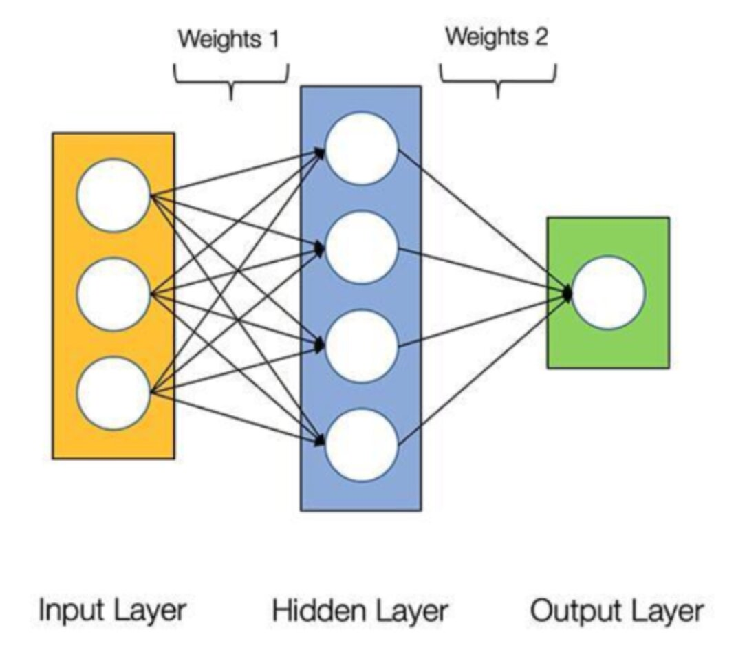
• Weight1 -> shape: 3 4
  Weight2 -> shape: 4 1

# Pytorch already implemented the simple feed forward network called "Linear"
# Input->Hidden
MLP1 = torch.nn.Linear(3,4)     #nn.Linear(input_dim, output_dim)
MLP1.weight, MLP1.bias

# Hidden->Output
MLP2 = torch.nn.Linear(4,1)
MLP2.weight, MLP2.bias

• feed forward network -> torch.nn.Linear(input_dim, output_dim) 형태로 구현이 가능함

x = torch.tensor([1., 0., 1.]) #input data
target = torch.tensor(0.5) #target data

## Pytorch has famous many used loss function and optimization
optim = torch.optim.SGD([MLP1.weight, MLP2.weight, MLP1.bias, MLP2.bias], lr=0.1) #Stochastic Gradient Descent

loss_func = torch.nn.MSELoss()

y = MLP1(x)
y = torch.nn.functional.sigmoid(y) # Activation function
y = MLP2(y)
y = torch.nn.functional.sigmoid(y) # Activation function
print("y value before update : ", y)

for i in range(10000):
  y = MLP1(x)
  y = torch.nn.functional.sigmoid(y)
  y = MLP2(y)
  y = torch.nn.functional.sigmoid(y)
  loss = loss_func(y, target)
  # pytorch automatically calculates the gradient and applies EBP(Error Back Propagation)
  optim.zero_grad()     # zero_grad() function is making the gradient zero..this time is for initialization
  loss.backward()       # pytorch automatically calculates the gradient
  optim.step()          # update the weights
  
check_y = MLP1(x)
check_y = torch.nn.functional.sigmoid(check_y)
check_y = MLP2(check_y)
check_y = torch.nn.functional.sigmoid(check_y)
MLP1.weight, MLP2.weight, check_y
# Weight of MLP1 layer and MLP2 layer has changed
# y value after update has changed to the target value

• x는 input data, target은 target data
• optimization은 torch.optim.SGD([MLP1.weight, MLP2.weight, MLP1.bias, MLP2.bias], lr=0.1)을 통해 Stochastic Gradient Descent을 방식을 사용
• loss_function은 torch.nn.MSEloss()를 사용함
• for문 위는 init 단계
• for문을 돌며 epochs: 10000번을 반복하여 training
• • zero_grad()를 통해 gradient를 초기화
• • loss.backward()를 통해 gradient 계산
• • optim.step()을 통해 weights값 갱신

class Two_layer(torch.nn.Module): # we inherited the torch module class
# we have to define __init__ function and forward function
  def __init__(self):
    super(Two_layer, self).__init__()
    # Initialize the layers 
    self.MLP1 = torch.nn.Linear(3, 4)
    self.MLP2 = torch.nn.Linear(4, 1)

  def forward(self, x): # x will be the input data
    y = self.MLP1(x)
    y = torch.nn.functional.sigmoid(y)
    y = self.MLP2(y)
    y = torch.nn.functional.sigmoid(y)
    return y

• 앞에서 했던 과정에서 model을 Two_layer class로 재구현

model = Two_layer()
x = torch.tensor([1., 0., 1.]) # input data
target = torch.tensor(0.5) # target data

## Pytorch implemented famous many used loss function and optimization
optim = torch.optim.SGD(model.parameters(), lr=0.1) # .parameters() contain all the learnable parameters on model defined on __init__ function (MLP1.weight, MLP2.weight, MLP1.bias, MLP2.bias])
loss_func = torch.nn.MSELoss()

for i in range(10000):
  y = model(x)
  loss = loss_func(target, y)
  optim.zero_grad()
  loss.backward()
  optim.step()
check_y = model(x)
check_y

• Stochastic Gradient Descent를 통해 optimization 진행
• loss_function은 마찬가지로 torch.nn.MSEloss()를 사용

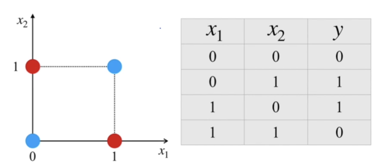
• 2 MLP layers를 사용해 XOR problem 해결 -> 2-dim input, 2-dim hidden, 1-dim output

class XOR_layer(torch.nn.Module):
  def __init__(self):
    super(XOR_layer, self).__init__()
    ## define your own layers!
    # Initialize the layers 
    self.MLP1 = torch.nn.Linear(2, 2)
    self.MLP2 = torch.nn.Linear(2, 1)
  
  def forward(self, x):
    # define the forward function
    y = self.MLP1(x)
    y = torch.nn.functional.sigmoid(y)
    y = self.MLP2(y)
    y = torch.nn.functional.sigmoid(y)

    return y

model = XOR_layer()
loss_func = torch.nn.MSELoss()
optim = torch.optim.SGD(model.parameters(), lr=0.1) 

### define x and target data
### for example, if x = [0, 0] --> target = [0] / x = [1, 0] --> target = [1]
### make 4 input as one input data
### for example, x = [[0,0], [1,0]] is 2 input data

x = torch.tensor([[0.,0.], [1.,0.], [0.,1.], [1.,1.]]) # input data
target = torch.tensor([[0.], [1.], [1.], [0.]]) # target data
for i in range(30000): # choose your own number of epochs
  y = model(x)
  loss = loss_func(target, y)
  optim.zero_grad()
  loss.backward()
  optim.step()
check_y = model(x)
check_y

• for문을 30000 epochs만큼 돌면서 model의 weights값 갱신
• check_y = model(x)을 통해 model이 잘 학습되었는 지 확인
• • 같은 데이터로 test하는 게 좀 이상하긴 함 -> train dataset과 test dataset을 분리해야함

# We will use 'Survived' feature as a class(y) but there is no 'Survived' feature in test.csv.
# So Split the train data into train and test data.

train = pd.read_csv(io.BytesIO(uploaded['train.csv']))
train, test = train_test_split(train, test_size = 0.3, random_state = 55)

# We dropped Cabin, name, ticket features because there are many null values and it's correlation with survived feature is low
train.drop(columns = ['PassengerId', 'Name', 'Ticket', 'Cabin'], inplace = True)

# We filled the null value of Embarked data with the most frequently used data
train['Embarked'].fillna(train['Embarked'].mode()[0], inplace = True) #pandas의 .mode() -> 최빈값을 구하는 메서드

• .mode() -> 최빈값을 구하는 method
• Embarked Column의 null 값을 최빈값으로 채움

# We filled the null value of age divided with the pclass. pclass and age has high correlation shown on the heatmap above! 
train['Age'].fillna(10000, inplace=True)
train.loc[(train['Pclass'] == 1) & (train['Age'] == 10000), 'Age'] = train.loc[(train['Pclass'] == 1) & (train['Age']!= 10000)]['Age'].mean()
train.loc[(train['Pclass'] == 2) & (train['Age'] == 10000), 'Age'] = train.loc[(train['Pclass'] == 2) & (train['Age']!= 10000)]['Age'].mean()
train.loc[(train['Pclass'] == 3) & (train['Age'] == 10000), 'Age'] = train.loc[(train['Pclass'] == 3) & (train['Age']!= 10000)]['Age'].mean()

• Pclass와 Age는 correlation이 높기 때문에, Pclass 별 age의 평균으로 age의 null 값을 채움

#one hot encoding
train = pd.get_dummies(train, columns = ['Sex'])
train = pd.get_dummies(train, columns = ['Embarked'])

• pd.get_dummies(train, columns = ['Column명']를 통해 지정한 Column의 값을 one hot encoding 해줄 수 있음
• MLP model에서 categorical 변수를 처리하기 위해 One-Hot Encoding을 사용하는 것은 모델의 성능을 향상시키고, categorical 변수의 정보를 적절하게 활용하기 위함임

# min max scailing -> Perceptron의 Input data는 이런식으로 가공해줘야함
min_age, max_age = train['Age'].min(), train['Age'].max()
min_fare, max_fare = train['Fare'].min(), train['Fare'].max()
min_pclass, max_pclass = train['Pclass'].min(), train['Pclass'].max()
train['Age'] = (train['Age'] - min_age) / (max_age  - min_age)
train['Fare'] = (train['Fare'] - min_fare) / (max_fare - min_fare)
train['Pclass'] = (train['Pclass'] - min_pclass) / (max_pclass - min_pclass)

• min, max scaling을 통해, 모든 값들이 0 ~ 1 사이의 값을 갖을 수 있도록 해줌

# We do the same data processing to the test dataset
# This is answer

# We dropped Cabin, name, ticket features because there are many null values and it's correlation with survived feature is low
test.drop(columns = ['PassengerId', 'Name', 'Ticket', 'Cabin'], inplace = True)

# We filled the null value of Embarked data with the most frequently used data
test['Embarked'].fillna(test['Embarked'].mode()[0], inplace = True)
# We filled the null value of age divided with the pclass. pclass and age has high correlation shown on the heatmap above! 
test['Age'].fillna(10000, inplace=True)
test.loc[(train['Pclass'] == 1) & (test['Age'] == 10000), 'Age'] = test.loc[(test['Pclass'] == 1) & (test['Age']!= 10000)]['Age'].mean()
test.loc[(test['Pclass'] == 2) & (test['Age'] == 10000), 'Age'] = test.loc[(test['Pclass'] == 2) & (test['Age']!= 10000)]['Age'].mean()
test.loc[(test['Pclass'] == 3) & (test['Age'] == 10000), 'Age'] = test.loc[(test['Pclass'] == 3) & (test['Age']!= 10000)]['Age'].mean()
test.isnull().sum()
#one hot encoding
test = pd.get_dummies(test, columns = ['Sex'])
test = pd.get_dummies(test, columns = ['Embarked'])

# min max scailing
min_age, max_age = test['Age'].min(), test['Age'].max()
min_fare, max_fare = test['Fare'].min(), test['Fare'].max()
min_pclass, max_pclass = test['Pclass'].min(), test['Pclass'].max()
test['Age'] = (test['Age'] - min_age) / (max_age  - min_age)
test['Fare'] = (test['Fare'] - min_fare) / (max_fare - min_fare)
test['Pclass'] = (test['Pclass'] - min_pclass) / (max_pclass - min_pclass)

test.to_csv('train_preprocessed.csv', index=False)
x_test = test.drop(columns='Survived')
y_test = test['Survived']
test

• test dataset에 대해서도 똑같이 data들을 전처리해줌

# Prepare your data for training with DataLoaders
x_train = torch.tensor(x_train.to_numpy(), dtype=torch.float32) # we can also use torch.from_numpy(x_train)
y_train = torch.tensor(y_train.to_numpy(), dtype=torch.float32)
y_train = y_train.reshape(-1,1) # -1 is used only once to indicate the remainder. ex) (24, 1) --> (-1, 4, 3) ==> -1 becomes 2
x_test = torch.tensor(x_test.to_numpy(), dtype=torch.float32)
y_test = torch.tensor(y_test.to_numpy(), dtype=torch.float32)
y_test = y_test.reshape(-1,1)

• data들을 tensor로 변경
• reshape(-1, 1)을 통해 행의 크기를 유지하면서 열의 크기를 1로 변경

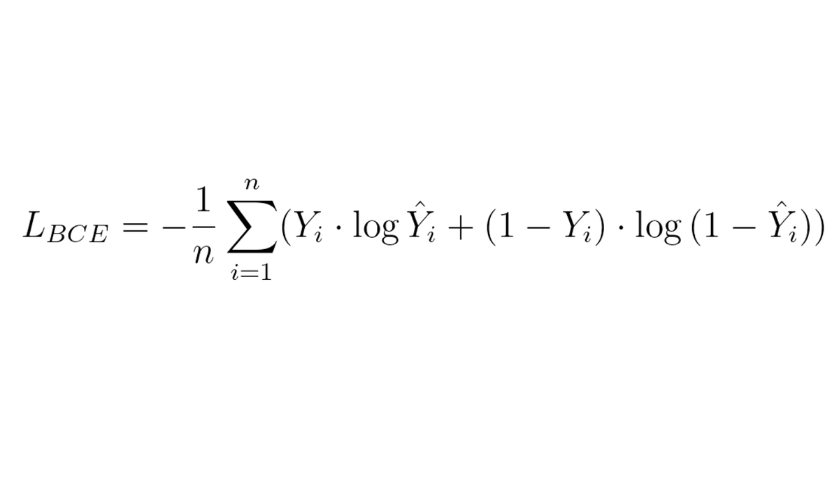
• Classification에선 MSE loss function을 사용할 수 없음 -> Cross Entrophy loss function을 사용해야함
• Yi는 target value, Yi_hat은 predicted value
• loss_function = torch.nn.BCELoss()를 통해 구현 가능

train = TensorDataset(x_train, y_train)
train_dataloader = DataLoader(train, batch_size = 64, shuffle=True)
test = TensorDataset(x_test, y_test)
test_dataloader = DataLoader(test, batch_size = 64, shuffle=False)

class Titanic_layer(torch.nn.Module):
  def __init__(self):
    super(Titanic_layer, self).__init__()
    
    ## define your own layers! 
    # Initialize the layers 
    
    self.MLP1 = torch.nn.Linear(10, 64)
    self.MLP2 = torch.nn.Linear(64, 32)
    self.MLP3 = torch.nn.Linear(32, 1)

  def forward(self, x):
    # define the forward function
    y = self.MLP1(x)
    y = torch.nn.functional.sigmoid(y)
    y = self.MLP2(y)
    y = torch.nn.functional.sigmoid(y)
    y = self.MLP3(y)
    y = torch.nn.functional.sigmoid(y)
    
    return y

• input features는 10임 -> (10, 64) -> (64, 32) -> (32, 1)로 layer 구성

# If you defined our model, you can just run this cell and next cell to check the accuracy of your model
epoches =  1000      # please write your own epoch
model = Titanic_layer()
optim = torch.optim.SGD(model.parameters(), lr = 0.05)
batch_len = len(train_dataloader)
for epoch in range(1, epoches+1):
  mean_loss = 0
  for i, data in enumerate(train_dataloader):
    x, target = data
    x = torch.tensor(x, dtype=torch.float32)
    y = model(x)
    target = torch.tensor(target, dtype=torch.float32)
    loss = loss_func(y, target)
    mean_loss += loss
    optim.zero_grad()
    loss.backward()
    optim.step()
  mean_loss /= batch_len
  print(f'Epoch: {epoch}, Train Loss: {mean_loss}')

• Stochastic Gradient Descent로 optimization
• loss function은 Cross Entrophy loss function을 사용