딥러닝 - 학습 규제 전략(Regularization Strategies)

‍Juhee Kim·2021년 7월 4일

Regularization Strategies 가중치 감소 가중치 제약 드롭아웃 딥러닝 학습규제전략

Deep Learning

목록 보기

5/7

오버피팅 (Overfitting)

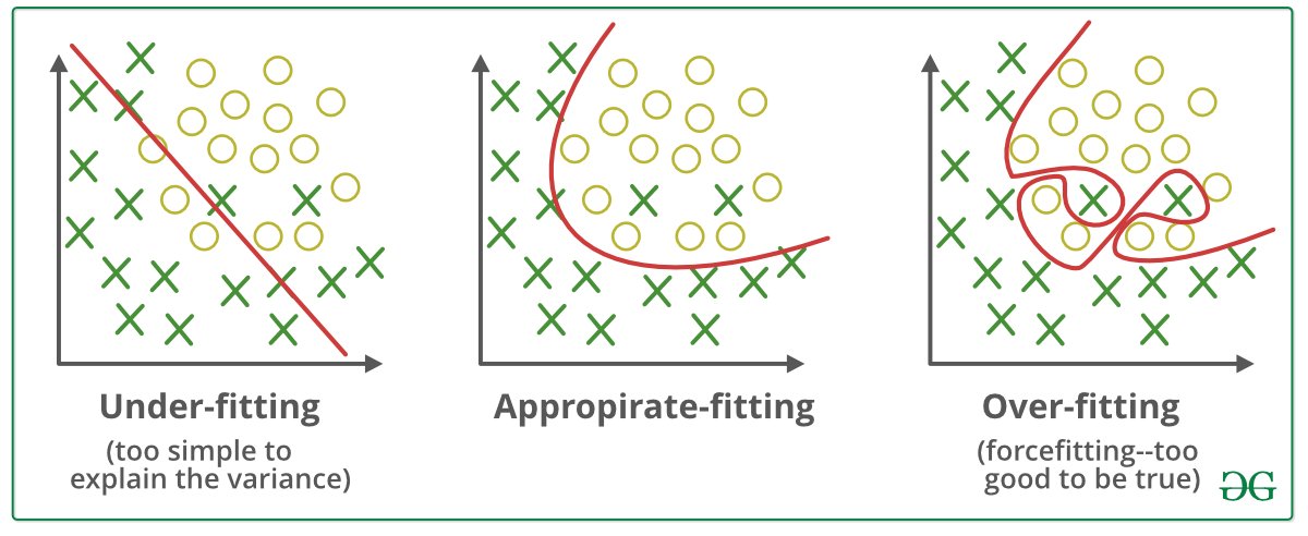
훈련 데이터에만 지나치게 적응되어 그 외의 데이터에는 제대로 대응하지 못하는 상태

오버피팅은 주로 다음의 두 가지 경우에 일어난다.

매개변수가 많고 표현력이 높은 모델(ex. 신경망)
훈련 데이터가 적을 때

과적합을 줄이기 위해 끊임없이 노력하는데, 이 문제를 해결하는 가장 중요한 방법은 가중치 규제 전략이다.

✨ 학습 규제 전략 (Regularization Strategies)

우리가 간단히 다루는 신경망에는 네 가지 일반적인 가중치 규제 방법이 있다.
이러한 구성요소를 적용하는 방법은 :

항상 EarlyStopping을 사용한다. 이 전략은 당신의 가중치의 최고 유용성 시점을 훨씬 지나서 더 업데이트되는 것을 막을 것이다.
EarlyStopping, 가중치 감소(Weight Decay) 및 Dropout 사용
EarlyStopping, 가중치 제약(Constraint) 및 Dropout 사용

Weight Decusion and Weight Restriction은 유사한 목적을 위하여 가중치를 제거하거나 값을 규제하여 매개변수를 과도하게 적합시키는 것을 방지하는 역할이다.
같은 목적의 다른 방법이기 때문에 이들을 굳이 같이 적용하지 않아도 된다.

✅ 가중치 감소 (Weight Decay)

학습 과정에서 큰 가중치에 대해서는 그에 상응하는 큰 패널티를 부과하여 오버피팅을 억제하는 방법

Weight Decay를 통해서 Weight의 학습 반경을 변경시킨다.

# Weight Decay를 전체적으로 반영한 예시 코드
from tensorflow.keras.constraints import MaxNorm
from tensorflow.keras import regularizers

# 모델 구성을 확인합니다.
model = Sequential([
    Flatten(input_shape=(28, 28)),
    Dense(64, input_dim=64,
            kernel_regularizer=regularizers.l2(0.01),     # L2 norm regularization
            activity_regularizer=regularizers.l1(0.01)),  # L1 norm regularization
    Dense(10, activation='softmax')
])

✅ 가중치 제약 (Constraints)

물리적으로 Weight의 크기를 제한하는 방법

Weight자체를 함수를 이용하여 더 큰 경우는 임의의 값으로 변경해버리는 기술을 사용한다. 그렇게 되면 값이 더 이상 커질 수 없을 것이다.

# 모델 구성을 확인합니다.
model = Sequential([
    Flatten(input_shape=(28, 28)),
    Dense(64, input_dim=64,
            kernel_regularizer=regularizers.l2(0.01),
            activity_regularizer=regularizers.l1(0.01),
            kernel_constraint=MaxNorm(2.)),  ## add constraints
    Dense(10, activation='softmax')
])

✅ 드롭아웃 (Dropout)

뉴런을 임의로 삭제하면서 학습시키는 방법

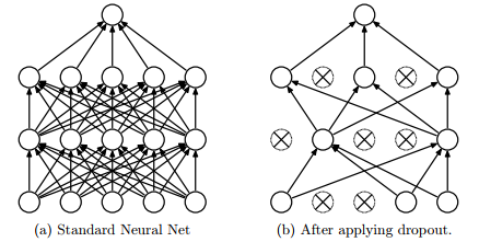
훈련 때 은닉층의 뉴런을 무작위로 골라 삭제한다. 삭제된 뉴런은 위의 그림과 같이 신호를 전달하지 않게 된다. 시험 때는 모든 뉴런에 신호를 전달한다. 단, 시험 때는 각 뉴런의 출력에 훈련 때 삭제 안 한 비율을 곱하여 출력한다.

from tensorflow.keras.layers import Dropout
from tensorflow.keras.constraints import MaxNorm
from tensorflow.keras import regularizers

# 모델 구성을 확인합니다.
model = Sequential([
    Flatten(input_shape=(28, 28)),
    Dense(64, input_dim=64,
            kernel_regularizer=regularizers.l2(0.01),
            activity_regularizer=regularizers.l1(0.01),
            kernel_constraint=MaxNorm(2.)),             
    Dropout(0.5),  ## add dropout
    Dense(10, activation='softmax')
])

※ 참고 ) 좀 더 나은 모델 학습을 위해 !

무엇인가 추가하는 방법이 아니라, 기존의 방법을 어떻게 활용할 지에 대한 고민

Learning rate decay

코드 예시

tf.keras.optimizers.Adam(
    learning_rate=0.001, beta_1=0.9, beta_2=0.999, epsilon=1e-07, amsgrad=False,
    name='Adam'
)

model.compile(optimizer=tf.keras.optimizers.Adam(lr=0.001, beta_1 = 0.89)
             , loss='sparse_categorical_crossentropy'
             , metrics=['accuracy'])

learning rate 스케쥴링

코드 예시

lr_schedule = keras.optimizers.schedules.ExponentialDecay(
    initial_learning_rate=1e-2,
    decay_steps=10000,
    decay_rate=0.9)

model.compile(optimizer=tf.keras.optimizers.Adam(learning_rate=lr_schedule)
             , loss='sparse_categorical_crossentropy'
             , metrics=['accuracy'])