Ch. 8 Deep Learning

8-7) Introduction to Keras

Preprocessing

• Tokenizer() : 토큰화와 정수 인코딩을 위해 사용됨

tokenizer = Tokenizer()
fit_text = "The earth is an awesome place live"
tokenizer.fit_on_texts([fit_text])

test_text = "The earth is an great place live"    # great은 단어집합에 없으므로 출력 X
sequences = tokenizer.texts_to_sequences([test_text])[0]

print("정수 인코딩 : ",sequences)
print("단어 집합 : ",tokenizer.word_index)

• pad_sequence() : 각 샘플의 길이를 동일하게 맞춰주는 패딩(padding)작업을 위해 사용됨

pad_sequences([[1, 2, 3], [3, 4, 5, 6], [7, 8]], maxlen=3, padding='pre')

Word Embedding

• 워드 임베딩: 텍스트 내의 단어들을 밀집벡터(dense vector)로 만드는 것
• 원-핫 벡터: 대부분 0의 값을 가지고, 단 하나의 1의 값을 가지는 벡터

-	원-핫 벡터	임베딩 벡터
차원	고차원 (단어집합의 크기)	저차원
다른 표현	희소 벡터의 일종	밀집 벡터의 일종
표현 방법	수동	훈련 데이터로부터 학습합
값의 타입	1 & 0	실수

• Embedding() : 단어를 밀집 벡터로 만드는 작업을 위해 사용됨.
  - 인공신경망 용어로는 '임베딩 층(embedding layer)을 만드는 역할'
  • input: (number of samples, input_length)인 2D 정수 텐서
    • sample: 정수 인코딩된 결과, 정수의 시퀀스
      - return값: (number of samples, input_length, embedding word dimensionality)인 3D 텐서
  • 인자
    • 첫번째 인자: 단어 집합의 크기. 총 단어의 개수
      • 두번째 인자: 임베딩 벡터의 출력 차원. 결과로서 나오는 임베딩 벡터의 크기
      • input_length: 입력 시퀀스의 길이

# 1. 토큰화
tokenized_text = [['Hope', 'to', 'see', 'you', 'soon'], ['Nice', 'to', 'see', 'you', 'again']]

# 2. 각 단어에 대한 정수 인코딩
encoded_text = [[0, 1, 2, 3, 4],[5, 1, 2, 3, 6]]

# 3. 위 정수 인코딩 데이터가 아래의 임베딩 층의 입력이 된다.
vocab_size = 7
embedding_dim = 2
Embedding(vocab_size, embedding_dim, input_length=5)

# 각 정수는 아래의 테이블의 인덱스로 사용되며 Embeddig()은 각 단어에 대해 임베딩 벡터를 리턴한다.
+------------+------------+
|   index    | embedding  |
+------------+------------+
|     0      | [1.2, 3.1] |
|     1      | [0.1, 4.2] |
|     2      | [1.0, 3.1] |
|     3      | [0.3, 2.1] |
|     4      | [2.2, 1.4] |
|     5      | [0.7, 1.7] |
|     6      | [4.1, 2.0] |
+------------+------------+
# 위의 표는 임베딩 벡터가 된 결과를 예로서 정리한 것이고 Embedding()의 출력인 3D 텐서를 보여주는 것이 아님.

Modeling

• Sequential() : 인공 신경망의 층을 구성하기 위해 사용됨.

from tensorflow.keras.models import Sequential
from tensorflow.keras.layers import Dense

model = Sequential()
model.add(층 이름 1) # 층 추가
model.add(층 이름 2) # 층 추가
model.add(층 이름 3) # 층 추가

model.add(Embedding(vocab_size, output_dim, input_length)) # 임베딩 층 추가

• Dense() : 전결합층(fully-connected layer)을 추가하기 위해 사용됨.
  - 인자
  - 첫번째 인자: 출력 뉴런의 수
  - input_dim: 입력 뉴런의 수 (입력의 차원)
  - activation: 활성화함수
  - linear: 디폴트값으로 별도 활성화함수 없이 입력 뉴런과 가중치 계산 결과 그대로 출력 ex. 선형 회귀
  - sigmoid, softmax, relu: 다양한 종류의 활성화 함수

model.add(Dense(1, input_dim=3, activation='relu'))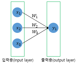

model = Sequential()
model.add(Dense(8, input_dim=4, activation='relu'))
model.add(Dense(1, activation='sigmoid')) # 출력층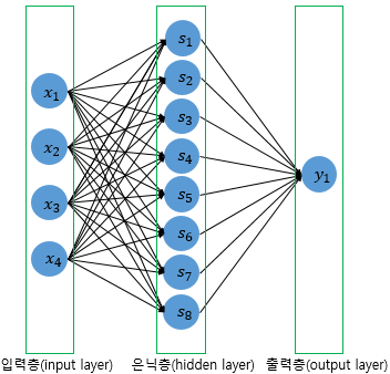

• summary(): 모델의 정보를 요약하여 보여줌.

model.summary()

_________________________________________________________________
Layer (type)                 Output Shape              Param #   
=================================================================
dense_1 (Dense)              (None, 8)                 40        
_________________________________________________________________
dense_2 (Dense)              (None, 1)                 9         
=================================================================
Total params: 49
Trainable params: 49
Non-trainable params: 0
_________________________________________________________________

Compile & Training

• compile(): 모델을 기계가 이해할 수 있도록 컴파일하기 위해 사용됨. 오차함수, 최적화방법, 메트릭 함수를 선택할 수 있음.
  - optimizer(): 훈련 과정을 설정하는 옵티마이저 설정
  - 'adam', 'sgd'와 같이 문자열로 지정 가능
  - loss: 훈련 과정에서 사용할 손실 함수 설정
  - metrics = 훈련을 모니터링하기 위한 지표 선택

# RNN을 이용한 이진 분류 코드 예시

from tensorflow.keras.layers import SimpleRNN, Embedding, Dense
from tensorflow.keras.models import Sequential

vocab_size = 10000
embedding_dim = 32
hidden_units = 32

model = Sequential()
model.add(Embedding(vocab_size, embedding_dim))
model.add(SimpleRNN(hidden_units))
model.add(Dense(1, activation='sigmoid'))
model.compile(optimizer='rmsprop', loss='binary_crossentropy', metrics=['acc'])

손실함수 & 활성화 함수 조합 예시

문제 유형	손실함수명	출력층의 활성화 함수명
회귀 문제	mean_squared_error(평균 제곱 오차)	-
다중 클래스 분류	categorical_crossentropy (범주형 교차 엔트로피)	softmax
다중 클래스 분류	sparse_categorical_crossentropy	softmax
이진분류	binary_crossentropy(이항 교차 엔트로피)	sigmoid

• fit(): 모델을 학습함.
  - 모델이 오차로부터 매개 변수를 업데이트 시키는 과정: 학습(learning), 훈련(training), 적합(fitting)
  • 인자
    • 첫번째 인자: 훈련 데이터
      • 두번째 인자: 지도학습에서의 label 데이터
      • epochs: 에포크. 정수값 기재 필요. 총 훈련 횟수
      • batch_size: 배치 크기. 기본값은 32. 미니 배치 경사 하강법 미 사용시 batch_size = None
      • validation_data(x_val, y_val): 검증 데이터 사용. 정확도 알려주나, 실제 모델이 검증 데이터를 학습하지는 않음. 검증 데이터의 loss가 낮아지다가 높아지기 시작하면 과적합(overfitting)의 신호임.
      • validation_split: validation_data 대체 가능. 별도의 검증 데이터를 주는 것이 아니라 스스로 일정 비율을 train data set에서 분리하여 검증 데이터로 사용. 마찬가지로 해당 데이터를 학습하지는 않음.
      • verbose: 학습 중 출력되는 문구
        - 0: 아무것도 출력하지 않음.
        • 1: 훈련의 진행도를 보여주는 진행 막대를 보여줌.
        • 2: 미니 배치마다 손실 정보를 출력합니다.

# 위의 compile() 코드의 연장선상인 코드
model.fit(X_train, y_train, epochs=10, batch_size=32)

# validation_data 사용
model.fit(X_train, y_train, epochs=10, batch_size=32, verbose=0, validation_data(X_val, y_val))

# validation_split 사용
# 훈련 데이터의 20%를 검증 데이터로 사용.
model.fit(X_train, y_train, epochs=10, batch_size=32, verbose=0, validation_split=0.2))

Evaluation & Prediction

• evaluate(): 테스트 데이터를 통해 모델에 대한 정확도 평가
  - 인자
  - 첫번째 인자: test data (x)
  - 두번째 인자: label test data (y)
  - batch_size: 배치 크기
• predict(): 임의의 입력에 대한 모델의 출력값 확인.
  - 인자
  - 첫번째 인자: 예측하고자 하는 데이터
  - batch_size: 배치 크기
  

Save & Load the Model

• save(): 인공신경망 모델을 hdf5 파일에 저장.
• load_model(): 저장해둔 모델을 불러옴.

8-8) Keras Functional API

Introduction to Functional API

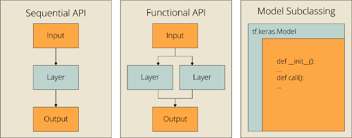
• Sequential API를 통한 방식으로는 층을 쌓는 것만으로는 구현할 수 없는 복잡한 신경망을 구현할 수 없음.
• Functional API는 각 층을 일종의 함수로 정의함.
• 입력의 크기 (shape)를 명시한 입력층(input layer)을 모델의 앞단에 정의해주어야만 함.

Fully-Connected FFNN

• 입력의 차원이 1인 전결합 피드 포워드 신경망(FFNN)

from tensorflow.keras.layers import Input, Dense
from tensorflow.keras.models import Model

inputs = Input(shape=(10,))

hidden1 = Dense(64, activation='relu')(inputs)
hidden2 = Dense(64, activation='relu')(hidden1)
output = Dense(1, activation='sigmoid')(hidden2)

model = Model(inputs=inputs, outputs=output)

model.compile(optimizer='rmsprop', loss='categorical_crossentropy', metrics=['accuracy'])
# model.fit(data, labels)

.
- 다른 변수명으로 구현된 FFNN

inputs = Input(shape=(10,))
x = Dense(8, activation="relu")(inputs)
x = Dense(4, activation="relu")(x)
x = Dense(1, activation="linear")(x)
model = Model(inputs, x)

• 선형 회귀 (Linear Regression)

from tensorflow.keras.layers import Input, Dense
from tensorflow.keras import optimizers
from tensorflow.keras.models import Model

X = [1, 2, 3, 4, 5, 6, 7, 8, 9] # 공부하는 시간
y = [11, 22, 33, 44, 53, 66, 77, 87, 95] # 각 공부하는 시간에 맵핑되는 성적

inputs = Input(shape=(1,))
output = Dense(1, activation='linear')(inputs)
linear_model = Model(inputs, output)

sgd = optimizers.SGD(lr=0.01)

linear_model.compile(optimizer=sgd ,loss='mse',metrics=['mse'])
linear_model.fit(X, y, epochs=300)

• 로지스틱 회귀 (Logistic Regression)

from tensorflow.keras.layers import Input, Dense
from tensorflow.keras.models import Model

inputs = Input(shape=(3,))
output = Dense(1, activation='sigmoid')(inputs)
logistic_model = Model(inputs, output)

• 다중 입력을 받는 모델 (Model that Accepts Multiple Inputs)

from tensorflow.keras.layers import Input, Dense, concatenate
from tensorflow.keras.models import Model

# 두 개의 입력층을 정의
inputA = Input(shape=(64,))
inputB = Input(shape=(128,))

# 첫번째 입력층으로부터 분기되어 진행되는 인공 신경망을 정의
x = Dense(16, activation="relu")(inputA)
x = Dense(8, activation="relu")(x)
x = Model(inputs=inputA, outputs=x)

# 두번째 입력층으로부터 분기되어 진행되는 인공 신경망을 정의
y = Dense(64, activation="relu")(inputB)
y = Dense(32, activation="relu")(y)
y = Dense(8, activation="relu")(y)
y = Model(inputs=inputB, outputs=y)

# 두개의 인공 신경망의 출력을 연결(concatenate)
result = concatenate([x.output, y.output])

z = Dense(2, activation="relu")(result)
z = Dense(1, activation="linear")(z)

model = Model(inputs=[x.input, y.input], outputs=z)

• RNN 은닉층 사용하기
  - 하나의 특성(feature)에 50개의 시점(time-step)을 입력으로 받는 모델 설계

from tensorflow.keras.layers import Input, Dense, LSTM
from tensorflow.keras.models import Model

inputs = Input(shape=(50,1))
lstm_layer = LSTM(10)(inputs)
x = Dense(10, activation='relu')(lstm_layer)
output = Dense(1, activation='sigmoid')(x)

model = Model(inputs=inputs, outputs=output)

8-9) Keras Subclassing API

Linear Regression with Subclassing API

import tensorflow as tf

class LinearRegression(tf.keras.Model):		# tf.keras.Model을 상속받음
  def __init__(self):	# 모델의 구조와 동적을 정의하는 생성자 정의 (속성값 초기화, 객체가 생성될때 자동으로 호출됨.)
    super(LinearRegression, self).__init__()	# tf.keras.Model의 속성을 가지고 초기화
    self.linear_layer = tf.keras.layers.Dense(1, input_dim=1, activation='linear')

  def call(self, x):	# 모델이 데이터를 입력받아 예측값을 리턴하는 포워드(forward) 연산 진행하는 함수
    y_pred = self.linear_layer(x)

    return y_pred
    
model = LinearRegression()

X = [1, 2, 3, 4, 5, 6, 7, 8, 9] # 공부하는 시간
y = [11, 22, 33, 44, 53, 66, 77, 87, 95] # 각 공부하는 시간에 맵핑되는 성적

sgd = tf.keras.optimizers.SGD(lr=0.01)
model.compile(optimizer=sgd, loss='mse', metrics=['mse'])
model.fit(X, y, epochs=300)

API Comparison

-	장점	단점
Sequential API	단순하게 층을 쌓는 방식. 쉬움. 긴딘힌 모델 구현하기 적합.	multi-input, multi-output을 가진 모델 or 층간의 연결(concatenate) or 덧셈(Add)와 같은 연산을 하는 모데을 구현하기에는 부적합.
Functional API	Sequential API로 구현할 수 없는 복잡한 모델 구현 가능. 대부분의 딥러닝 모델은 Functional API 수준에서도 전부 구현 가능함.	기본적으로 딥 러닝 모델을 DAG (Directed Acyclic Graph)로 취급. 재귀 네트워크, 트리 RNN 등은 이 가정을 따르지 않아 구현이 불가능함. 입력의 크기(shape)를 명시한 입력층(input layer)을 모델의 앞단에 정의해주어야함.
Subclassing API	Subclassing API로도 구현할 수 없는 복잡한 모델 구현 가능. 밑바닥부터 새로운 수준의 아키텍처를 구현해야하는 실험적 연구를 하는 연구자에게 적합함.	객체지향 프로그래밍에 익숙해야함. 코드 사용이 가장 까다로움.

8-10) Text Classification with MultiLayer Perceptron (MLP)

Introduction to MLP

• 단층 퍼셉트론 형태에서 은닉층이 1개 이상 추가된 신경망
• 피드 포원드 신경망 (FFNN)의 가장 기본적인 형태
• 한 방향(입력층 -> 출력층)으로만 연산 방향이 정해져 있는 신경망

texts_to_matrix() of Keras

텍스트 데이터로부터 행렬(matrix)를 만드는 도구

import numpy as np
from tensorflow.keras.preprocessing.text import Tokenizer

texts = ['먹고 싶은 사과', '먹고 싶은 바나나', '길고 노란 바나나 바나나', '저는 과일이 좋아요']

tokenizer = Tokenizer()
tokenizer.fit_on_texts(texts)
print(tokenizer.word_index)

below is the result

{'바나나': 1, '먹고': 2, '싶은': 3, '사과': 4, '길고': 5, '노란': 6, '저는': 7, '과일이': 8, '좋아요': 9}

texts_to_matrix에는 4개의 모드가 있음.

• count
  - 문서 단어 행렬(DTM)을 생성함.
  • DTM의 인덱스는 위의 word_index의 결과임.
  • Bag of Words(BoW) 기반이기 때문에 단어 순서 정보는 보존되지 않음. (4개의 모든 모드에서 해당 정보는 보존되지 않음.)

print(tokenizer.texts_to_matrix(texts, mode = 'count')) # texts_to_matrix의 입력으로 texts를 넣고, 모드는 'count'

below is the result

[[0. 0. 1. 1. 1. 0. 0. 0. 0. 0.]
 [0. 1. 1. 1. 0. 0. 0. 0. 0. 0.]
 [0. 2. 0. 0. 0. 1. 1. 0. 0. 0.]
 [0. 0. 0. 0. 0. 0. 0. 1. 1. 1.]]

• binary
  - 단어의 유무만 관심을 가지고, 개수는 고려하지 않음.

print(tokenizer.texts_to_matrix(texts, mode = 'binary'))

below is the result

[[0. 0. 1. 1. 1. 0. 0. 0. 0. 0.]
 [0. 1. 1. 1. 0. 0. 0. 0. 0. 0.]
 [0. 1. 0. 0. 0. 1. 1. 0. 0. 0.]
 [0. 0. 0. 0. 0. 0. 0. 1. 1. 1.]]

• tfidf
  - TF-IDF 행렬을 만듦.
  • TF: 각 문서에서 각 단어의 빈도에 자연로그를 씌우고 1을 더한 값
  • IDF: 기본식에서 로그를 자연 로그로 사용하고, 로그 안의 분수에 1을 추가

print(tokenizer.texts_to_matrix(texts, mode = 'tfidf').round(2)) # 둘째 자리까지 반올림하여 출력

below is the result

[[0.   0.   0.85 0.85 1.1  0.   0.   0.   0.   0.  ]
 [0.   0.85 0.85 0.85 0.   0.   0.   0.   0.   0.  ]
 [0.   1.43 0.   0.   0.   1.1  1.1  0.   0.   0.  ]
 [0.   0.   0.   0.   0.   0.   0.   1.1  1.1  1.1 ]]

• freq
  - (각 문서에서의 각 단어의 등장 횟수) / (각 문서의 크기 = 각 문서에서 등장한 모든 단어의 개수의 총합)

8-11) Neural Network Language Model (NNLM)

The Limitation of N-gram

희소 문제 (sparsity problem): 충분한 데이터를 관측하지 못하면 언어를 정확히 모델링할 수 없음.

Word Similarity

단어간 유사도를 반영하면 기존의 데이터에 없던 조합도 쉽게 만들고 학습할 수 있음.

Feed Forward NNLM

NNLM은 N-gram과 동일하게 전체 단어가 아닌 정해진 n개의 단어만을 참고함.
이때 해당하는 범위를 '윈도우(Window)'라고 부름.

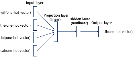
NNLM은 위와 같이 총 4개의 층으로 구성되어있음.
input layer에서는 window 크기만큼 입력이 들어옴.
- 해당 값은 각 단어의 원-핫 벡터임.

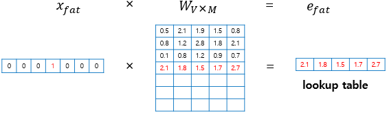
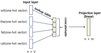
투사층:

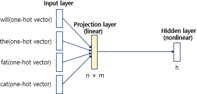
은닉층:

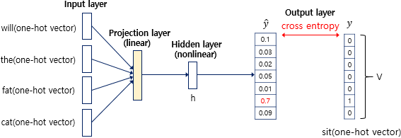
출력층:

Performance of NNLM

• 장점:
  - 밀집 벡터 사용 -> 단어 유사도 표현 가능 -> 희소 문제 해결
  • 모든 n-gram 저장할 필요가 없음. n-gram보다 저장공간에서의 이점을 지님.
• 단점:
  - 정해진 n개의 단어 참고 -> 버려지는 단어들이 가진 문맥 정보는 참고할 수 없음.
  • 각 문장의 길이는 전부 다를 수 있으므로 모델이 매번 다른 길이의 입력 시퀀스에 대해서도 처리할 수 있어야함.
  • 피드 포워드 신경망으로 만든 언어모델이 이를 수행하는 것이 어려우니 다른 신경망을 사용하여야함.