Ch. 4 Count Based Word Representation

4-1) Other Word Representation Methods

Introduction to Word Representation

There are two types of word representation:

1. Local Representation (=Discrete Representation)
   :Referencing the word only, and map specific value
   -> It cannot entail nuance of the word

2. Distributed Representation (=Continuous Representation)
   :Referencing surroundings of the word, and express it
   -> It can entail nuance of the word

Category of Word Representation

Bag of Words (=BoW) is Local Representation method.
It counts the frequency of the word, and quantify it.

4-2) Bag of Words (BoW)

Introduction to BoW

BoW does not consider the order of words, but only focuses on frequency of it.
Below is the simplified mechanism of BoW.

1. We assign specific int index to each word.
2. We create vector that records the frequency of the word token in each index.

4-3) Document-Term Matrix (DTM)

Introduction to DTM

If we switch row and column, we call it TDM.
It is a combination of BoWs from different documents into one matrix.

Limitation of DTM

It is simple, but has some limitation below.

1. Sparse Representation
   In One-Hot Vector, the size of vocabulary is the dimension of the vector. Therefore, most of the values are 0, which can increase calculation resource, and can cause spatial waste.
   DTM shares the same problem. The size of the entire vocabulary is the dimension of the vector for DTM.
   We call vectors with most of the values are 0 as 'sparse vector' or 'sparse matrix'.
   In order to reduce the size of vocabulary, it is important to preprocess and regularize words.

2. Limitation of Frequency Based Method
   There are both meaningful words and meaningless words. In order to prevent confusion made by meaningless words, we will a) remove stopwords, and b)give different weight for each word.
   We will use TF-IDF to do so.

4-4) Term Frequency-Inverse Document Frequency (TF-IDF)

Introduction to TF-IDF

If we can calculate importance of each word, we will be able to consider more information compared to using mere DTM.
Note. TF-IDF is not always better than DTM.

TF-IDF uses word frequency and inverse document frequency to weigh words differently by their importance. We create DTM first, then use TF-IDF weights.

It can be used for

• Calculating document similarity
• Calculating importance and priority of search results in search system
• Calculaitng importance of specific word in the document

Definition of Expressions of TF-IDF

d = document
t = word (term)
n = number of documents
tf = word frequency in DTM

tf(d,t) = frequency of word 't' in the document 'd'

df(t) = number of documents with the word 't'

• the frequency of word in each document is not considered

idf(d,t) = inverse of df(t)

• The reason why we use log:
  a) If we don't use log, the value of IDF will increase exponentially as 'n' increases
  b) If we don't use log, we might give excessive weight to rare words

• The reason why we add 1:
  a) If we don't do it, there can be a case with denominator as 0 if specific word does not exist in the entire document

Summary of TF-IDF

• TF-IDF considers the frequent word in the entire document is less important, and considers the frequent word in specific document is more important.
• If TF-IDF value is low, the importance is low, and vice versa.
• Stopwords' TF-IDF values are usually lower than other words'.
• We use natural logarithm for IDF. Its base is e. We express it as 'ln' instead of 'log'.
• If we multiply TF by IDF, we now have TF-IDF value.

Ch.5 Vector Similarity

5-1) Cosine Similarity

Introduction to Cosine Similarity

We can calculate document similarity using cosine similarity if words are quantified by BoW, DTM, TF-IDF, Word2Vec etc.

It signifies how similar the directions of two vectors are.

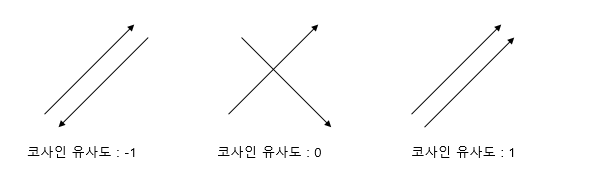
Using cosine angle,
a) if the directions of two vectors are same, cosine similairy is 1
b) if the angle of directions of two vectors is 90', cosine similarity is 0
c) if the angle of directions of two vectors is the opposite, cosine similarity is -1

Its range is -1 to 1.
Below is the formula of calculating cosine similarity for vector A and B.

If we do not use cosine similarity, longer document will have higher chance of getting higher similarity with other documents.

5-2) Various Similarity Methods

Euclidean Distance

It is not useful compared to Jaccard similarity nor cosine similarity.
In multi-dimensional space, when point 'p' and 'q' has coordination of

below is the formula of calculating euclidean distance

If we assume it as two-dimensional space,

Above is the visualized distance between two points in coordinate plane.

Jaccard Similarity

Its range is 0 to 1.
If two sets are the same, jaccard similarity is 1.
If two sets are disjoint sets, jaccard similarity is 0.

Below is the formula 'J' for calculating jaccard similarity between set 'A' and set 'B'.