사실상 이걸 이해하기 위하여 공업 수학 정리를 시작했다. 공학 전공이지만 문과 찍먹 공학 찍먹을 한 내 입장에서는 기본기가 정말 중요했다. Depth 있게 공부해보고자 한다.
Eigenvalue & Eigenvector
Definition
(Square matrix)
그렇다면, 는 의 eigenvalue라고 한다.
는 의 eigenvector라고 하며, eigenvalue와 eigenvector는 corresponding이 되어 있다. 그렇기에 무수히 많은 eigen value/vector 후보가 있는 와중에 아래 식이 성립이 되는 것이다.
이들의 관계식은 아래와 같이 표현하며 "Eigenvalue equation"이라고 한다.
이 식이 특이한 점은 A는 매트릭스( )
는 스칼라()이지만, 하나의 equation으로 표현할 수 있다는 것이다. 이러한 특이성을 만족하는 와 에 각각의 이름을 부여하는 것이다.
직관적인 예시를 들어보자.
를 projection matrix라고 생각한다면,
라는 점을 vector space로 projection시킨다는 것을 표현한 것이다.
시각화 해보자
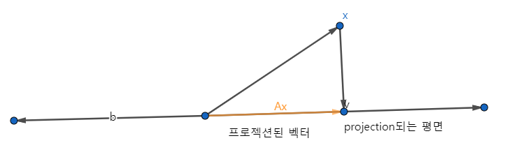
projection된 벡터 스페이스 상에서는 를 곱하면 방향이나 길이가 변화하는 것.
표기법으로는 eigenvalue가 큰 것부터 작은 것 순으로 sorting하여 표기한다.
Equivalent Statements
eigenvector와 eigenvalue가 존재한다면, Eigenvalue equation을 정리하여 아래의 식으로 전개 할 수 있다.
가 0이 아닌 솔루션이 존재하는 homogeneous equation이다. 그렇기에, non trivial solution이 존재한다고 표현한다.
그렇다면 x가 0이되면 안되므로 은 역행렬이 존재 하지 않아야만 한다. 이라는 의미이고, full rank matrix가 아니라는 의미이다. ()
Colinearity and Codirection
Cordirected
두 벡터가 같은 방향을 가리킬 경우, codirected 되었다고 한다.
Colinear
두 벡터가 정확히 똑같은 방향을 포인트하거나 정반대의 방향을 포인트 하는 경우 Colinear 관계에 있다고 한다.
응용하면, cordirected이면 colinear하게 되기도 한다.
Non-uniqueness of Eigenvectors
Definition
는 의 eigenvector이며
는 eigenvalue이다. 이 때, c는 0을 제외한 스칼라 값이라고 한다면,
(c) = c = c = (c)
로 수식을 변형 전개해 볼 수 있다.
특이한 점이 c는 다시 의 eigenvector가 되고, 는 여전히 같은 eigenvalue값을 갖는 것을 알 수 있다.
그러므로 에 "colinear"한 모든 벡터는 여전히 에 대한 eigenvetor라고 할 수 있다.
Eigenspace & Eigenspectrum
Eigenspace
일 때, eigenvalue에 대응되는 모든 eigenvector의 span한 generating set(subspace)를 eigenspace라고 한다.
- Notation
Eigenspectrum
모든 eigenvalue의 set을 가리킨다.
Properties of e-val. & e-vec
Properties
- 매트릭스 A에 transpose를 거쳐도 와 의 e-val은 동일하다. 단, e-vec은 꼭 동일하지는 않을 것이다.
- eigenspace 는 의 null space이다.
- Similar matrices는 같은 e-val을 갖는다. basis가 바뀌더라도 e-val값은 바뀌지 않는다. 그렇기 때문에 특정 고유값 역할을 할 수 있는 것이다. (e-val, det, trace 세 가지가 linear mapping에서 주요 파라미터이지만 그 중에서도 으뜸은 e-val이다. det, trace의 경우에는 matrix 하나당 한가지의 값만 나오게 된다. 반면, e-val의 경우 matrix A가 있을 경우 최대 n개 값의 조합이 생긴다. subspace를 표현하는 키값이 많을 수록 표현이 용이하므로 e-val이 subspace나 linear mapping을 더 잘 표현하는 키 파라미터가 된다.)
- Symmetric, positive definite matrix는 항상 양수이고, real 값을 갖는 e-val이 나온다.
Example for e-val & e-vec
의 와 를 구해보자.
if
if
두 가지 형태의 e-val, e-vec을 구할 수 있다.
Linear Independence & e-val
- 에서 매트릭스 A에 n개의 서로다른 e-val가 있을 때, 그 안에 있는 n개의 e-vec들은 linearly independent하다고 할 수 있다.
Defective (-하다)
서로 다른(독립성을 갖는) e-vec의 개수가 n보다 작을 때, 이 매트릭스를 defective한 매트릭스라고 표현한다. 이 경우 A매트릭스에 대해 Inverse를 계산할 수 없는 등 계산에 부적합한 matrix형태가 된다.
Symmetric & Semidefinite Matrix
- symmetric :
- Semi definite :
인 매트릭스 A가 있을 때,
를 만족한다면, "항상" symmetirc하고 positive semidefinite한 매트릭스 을 얻을 수 있다.
- symmetric? 를 아래에 대입해서 전개해보면 증명할 수 있다.
- semi definite?
나오므로 항상 0보다 크거나 같다.
혹은 이렇게 표현할 수도 있다.
이라면, 는 symmetric하고 positive definite하다.
Determinant & Trace & Eigenvalues
특성 subspace를 나타내기 위하여 3가지의 고유값을 찾는 것이다.
결국 e-val의 곱이 det이다. 이는 추후 Decomposition에서 활용될 중요한 개념이다.
diagonal 성분에 e-val이 위치되고 이를 곱하기만 하면 되는 것이다.
결국 e-val 의 합이 trace이다.
앞으로는 det, tr를 찾는 것이 아니라 eigenvalue와 eigenvector를 구하는 수준으로 내려오게 된 것이다.