
오늘은 회귀분석와 최소자승법에 대해서 배워보도록하겠습니다.
회귀분석(Resgression)
회귀 분석이란 데이터(x,y변수)에 대해 두 변수 사이의 모형을 구해 적합도를 측정하는 것입니다.
x값에 따라 y값을 정할 수 있는 경우 회귀분석을 쓰며, 이럴 때 x는 독립변수, y는 종속변수가 됩니다.
최소자승법(Least Square Method,LSM)
최소제곱법(Ordinary Least Square,OLS)
최소자승법과 최소제곱법은 같은 뜻이며, 어떤 모델의 파라미터를 구하는 방법 중 하나입니다. 이것은 데이터와의 residual^2(잔차의 제곱)의 합을 최소화하도록 모델의 파라미터를 구하는 방법입니다.
두가지다 글로써는 이해하기 어려우니 코드로 확인해보겠습니다.
회귀함수사용
input
from sklearn.datasets import make_regression
#n_samples 샘플수, n_features 독립변수의 수, bias 절편, noise 표준편차 , random_state 난수 발생용 시작값 , coef True면 선형 모형의 계수도 출력
X,y,coef=make_regression(n_samples=50, n_features=1, bias=100, noise=30, random_state=0, coef=True)
print(X[:5])
print(X[:5].flatten()) #2차원 배열을 1차원 배열로 변환
print(y[:5])
print(coef)
output
[[-0.85409574]
[ 1.49407907]
[-0.34791215]
[ 0.44386323]
[-0.18718385]][-0.85409574 1.49407907 -0.34791215 0.44386323 -0.18718385]
[ 34.65233505 142.34534472 51.1031876 86.80542038 127.56074762]
15.896958364551972
n_samples= 샘플 수(정수)
n_features= 독립변수의 수(차원,정수)
bias= y절편(실수)
noise=종속 변수에 더해지는 정규 분포의 표준편차(실수)
random_state=난수 발생용 시작값(정수)
coef=True
기본 선형 모델의 계수(기울기)를 설정해줍니다.이를 출력하면
X,y,coef(기울기)의 값을 얻을 수 있습니다.
데이터 등분
input
import numpy as np
xx=np.linspace(-3,3,100) #-3~3 100등분
y0=coef*xx+100 # 가중치(기울기) coef를 곱하고 절편 100을 더함
print(xx)
print(y0)
output
[-3. -2.93939394 -2.87878788 -2.81818182 -2.75757576 -2.6969697
-2.63636364 -2.57575758 -2.51515152 -2.45454545 -2.39393939 -2.33333333
-2.27272727 -2.21212121 -2.15151515 -2.09090909 -2.03030303 -1.96969697
-1.90909091 -1.84848485 -1.78787879 -1.72727273 -1.66666667 -1.60606061
-1.54545455 -1.48484848 -1.42424242 -1.36363636 -1.3030303 -1.24242424
-1.18181818 -1.12121212 -1.06060606 -1. -0.93939394 -0.87878788
-0.81818182 -0.75757576 -0.6969697 -0.63636364 -0.57575758 -0.51515152
-0.45454545 -0.39393939 -0.33333333 -0.27272727 -0.21212121 -0.15151515
-0.09090909 -0.03030303 0.03030303 0.09090909 0.15151515 0.21212121
...
129.38528667 130.3487387 131.31219072 132.27564274 133.23909476
134.20254678 135.16599881 136.12945083 137.09290285 138.05635487
139.01980689 139.98325892 140.94671094 141.91016296 142.87361498
143.83706701 144.80051903 145.76397105 146.72742307 147.69087509]
데이터의 정밀도를 올리기위해 등분 시켜줍니다.
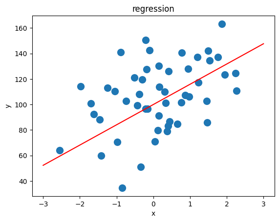
데이터 시각화
input
import matplotlib.pyplot as plt
plt.plot(xx,y0,'r-') #회귀선
plt.scatter(X,y,s=100) #산점도
plt.xlabel('x')
plt.ylabel('y')
plt.title('regression')
output
회귀함수로 데이터 만들기
input
from sklearn.datasets import make_regression
from sklearn.linear_model import LinearRegression
bias=100
X,y,coef=make_regression(n_samples=200, n_features=1, bias=bias, noise=10, coef=True, random_state=1)
model=LinearRegression().fit(X,y)
#절편,기울기
model.intercept_, model.coef_
output
(99.79150868986945, array([86.96171201]))
새로운 값 및 예측
input
#새로운 값을 입력하여 y 예측, 2차원 배열로 입력함
# y=86*-2 + 99
model.predict([[-2],[-1],[0],[1],[2]])
output
array([-74.13191534, 12.82979668, 99.79150869, 186.7532207 ,
273.71493272])
predict함수는 일반 함수(Generic Function)로 여러 가지 방식으로 모델을 만들었을 때 해당 모델로부터 새로운 데이터에 대한 예측값을 구하는 데 사용합니다.
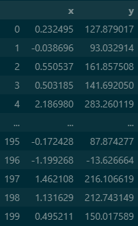
데이터프레임화
input
import pandas as pd
df=pd.DataFrame({'x':X.flatten(), 'y':y})
df
output
최소자승법 사용
input
import statsmodels.api as sm
X=df[['x']]
y=df[['y']]
model=sm.OLS(y,X) #최소자승법 함수
result=model.fit() # 학습
result.summary()
# R-squared (rvalue 결정계수) 0.0~1.0 모형의 설명력
output
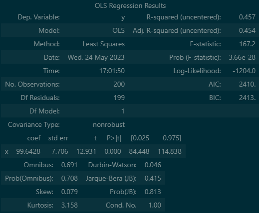
여기서 주의깊게 봐야 할 것은 R-squared이며, 이것은 모델이 얼마나 정확도를 가지는 지에대해 설명해 줍니다.예시로 해보았을뿐 45%는 설명력이 적은 편입니다.
또한 coef(회귀계수), P>|t|(p-value) 또한 이용하여 무엇이 문제 인지 확인 할 수 있습니다.
응용
input
#새로운 값 예측, 1차원 배열로 입력
print(result.predict([-2,-1,0,1,2]))
print(result.params)
output
[-199.28565959 -99.64282979 0. 99.64282979 199.28565959]
x 99.64283
dtype: float64
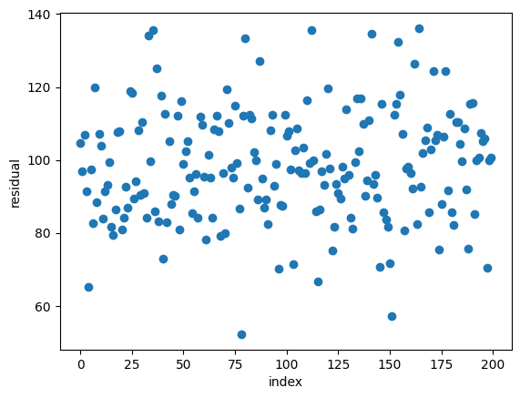
잔차확인
input
# 잔차: 실제값과 예측값의 차이
result.resid
output
0 104.712602
1 96.888644
2 107.000394
3 91.553292
4 65.343279
...
195 105.055511
196 105.871796
197 70.418046
198 99.984395
199 100.673331
Length: 200, dtype: float64
데이터 시각화
input
import matplotlib.pyplot as plt
result.resid.plot(style='o')
plt.xlabel('index')
plt.ylabel('residual')
plt.show()
#잔차 벡터 그래프
output
오늘은 데이터를 분석하는 방법중 최회귀분석의 최소자승법에 대해 배워 보았습니다. 데이터 분석방법은 여러가지가 있으니 하나하나 배워보려고 합니다.
😁 power through to the end 😁