
이번시간에는 지금까지 배운 것들을 활용하여 로지스틱회귀분석을 응용해보도록 하겠습니다.
데이터셋 생성
input
import random

def calc_bmi(h,w):
    bmi=w/(h/100)**2
    if bmi < 18.5: return '1'
    if bmi < 25: return '2'
    return '3'

fp=open('d:/data/bmi/bmi.csv','w',encoding='utf-8') # 디렉토리에 Write로 파일 오픈
fp.write('height,weight,label\n') # 작성
cnt={'1':0, '2':0, '3':0} # 각 label 갯수 초기화
for i in range(2000000): # 총 200만건
    h=random.randint(120,200) # 키를 120~200까지 랜덤 생성
    w=random.randint(35,80) # 몸무게를 35~80까지 랜덤 생성
    label=calc_bmi(h,w) # 각 라벨을 작성한 calc_bmi함수를 이용하여 구분
    cnt[label]+=1 # 갯수
    fp.write(f'{h},{w},{label}\n')
fp.close()
print(cnt,'건의 데이터가 생성되었습니다.')
output
{'1': 639854, '2': 592111, '3': 768035} 건의 데이터가 생성되었습니다.
파일을 열고 작성 및 저장하는 전에 배운 방법을 활용하여 bmi label 18.5이하는 1 25이하는 2 25초과는 3으로 하여 생성 해줍니다. 200만건의 데이터를 키는 120~200, 몸무게는 35~80으로 랜덤하게 생성합니다. 램덤 생성이기 때문에 매번 값이 다르게 생성됩니다.
데이터셋 데이터프레임화
input
import pandas as pd
df=pd.read_csv('d:/data/bmi/bmi.csv')
df.head()
output
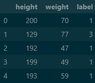
생성한 데이터셋을 pandas를 이용하여 데이터프레임화 시켜줍니다.
독립, 종속 변수 분할
input
train_cols=df.columns[:2]
X=df[train_cols]
y=df['label']
y.value_counts() # 갯수 카운트
output
label
3 768035
1 639854
2 592111
Name: count, dtype: int64
회귀분석을 하기 위해서 독립변수(X)와 종속변수(y)를 분할 해줍니다.
샘플링
input
from imblearn.under_sampling import RandomUnderSampler
X_sample,y_sample=RandomUnderSampler(random_state=0).fit_resample(X,y)
X_samp=pd.DataFrame(data=X_sample, columns=train_cols)
y_samp=pd.DataFrame(data=y_sample, columns=['label'])
df2=pd.concat([X_samp, y_samp],axis=1)
df2.label.value_counts()
output
label
1 592111
2 592111
3 592111
Name: count, dtype: int64
데이터 갯수의 편차가 있기 때문에 가장 적은 데이터를 기준으로 언더 샘플링을 해줍니다.
독립, 종속 변수 분할
input
X=X_samp[train_cols]
y=y_samp['label']
샘플링한 데이터를 다시 분할 해줍니다.
모델 학습
input
from sklearn.model_selection import train_test_split
from sklearn.linear_model import LogisticRegression
X_train,X_test,y_train,y_test=train_test_split(X,y,test_size=0.2,random_state=0, stratify=y)
model=LogisticRegression()
model.fit(X_train,y_train)
output

연습과 검증 케이스를 8:2 비율로 나누어 종속변수(y)를 기준으로 모델 학습을 해줍니다.
정확도 확인
input
print(model.score(X_train,y_train))
print(model.score(X_test,y_test))
output
0.9816820612132019
0.9819121956162549
예측하기
input
from sklearn.metrics import confusion_matrix
pred=model.predict(X_test) #모델 예측
confusion_matrix(y_test,pred) # 혼돈행렬으로 시각화
output
array([[116904, 1519, 0],
[ 1560, 115242, 1620],
[ 0, 1727, 116695]], dtype=int64)
predict를 이용하여 예측값을 구하고 confusion_matrix를 이용하여 시각화합니다.
평가하기
input
from sklearn.metrics import classification_report
print(classification_report(y_test,pred))
output
precision recall f1-score support
       1       0.99      0.99      0.99    118423
       2       0.97      0.97      0.97    118422
       3       0.99      0.99      0.99    118422

accuracy                           0.98    355267
macro avg      0.98      0.98      0.98    355267
weighted avg   0.98      0.98      0.98    355267
classification_report함수는 예측결과를 기반으로 분류 모델의 성능을 평가해주는 함수힙니다.
정밀도(precision), 재현율(recall), F1-score, 지원 개수(support) 등의 지표를 제공하여 모델의 성능을 종합적으로 평가할 수 있습니다.
오늘은 회귀함수를 배운것을 기반으로 최종 정리및 응용하는 방법을 배워보았습니다.제가 배운 분석은 데이터셋 작성 및 불러오기 -> 전처리 -> 학습 -> 평가를 기반을 기반으로 하고있습니다.
😁 power through to the end 😁