Python 전처리 자동화

Jayce_97·2023년 5월 29일

교차검증 자동화 전처리

Python 전처리

목록 보기

3/3

오늘은 전처리중 전처리중 최적의 파라미터를 선택하는 방법을 알아보려고 합니다.

데이터셋 불러오기

input

import pandas as pd 
from sklearn.datasets import fetch_openml
X,y=fetch_openml('titanic',version=1,as_frame=True,return_X_y=True)
df=pd.concat([X,y],axis=1)
df.head()

output

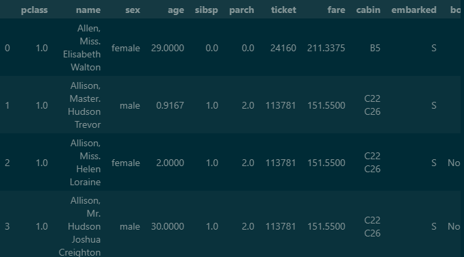
여러번 사용해본 titanic 데이터 셋을 불러오기 위해 fetch_openml을 사용해 줍니다.
as_frame과 return_X_y가 true로 설정시 DataFrame 또는 Series로 변환 시킬 수 있습니다.
fetch_openml 옵션 설명 링크에서 확인 할 수 있습니다.
만들어진 변수 X,y를 concat 을 이용하여 결합을 시켜줍니다.

독립, 종속변수 설정

input

train_cols=['pclass','sex','age','sibsp','parch','fare','embarked']
X=df[train_cols]
y=df['survived']
y.value_counts()

output

survived
0 809
1 500
Name: count, dtype: int64

pclass(숙소), sex(성별), age(나이)등이 survived(생존)에 대한 영향을 확인하기 위해 독립변수(X)와 종속변수(y)로 나누어 줍니다.

샘플링(Sampling)

input

from imblearn.under_sampling import RandomUnderSampler 
X_sample,y_sample=RandomUnderSampler(random_state=0).fit_resample(X,y)
X_samp=pd.DataFrame(data=X_sample, columns=train_cols)
y_samp=pd.DataFrame(data=y_sample, columns=['survived'])
df2=pd.concat([X_samp, y_samp], axis=1)
X=df2[train_cols]
y=df2['survived']
y.value_counts()

output

survived
0 500
1 500
Name: count, dtype: int64

언더샘플링(undersampling)은 다수 범주의 값들을 감소시키고 데이터 비율을 맞춰서 재현율을 향상시키는 샘플링 방법입니다.반대로 오버샘플링(oversampling)은 데이터를 증가시켜서 비율을 맞춥니다.
언더샘플링은 처리속도는 빠르지만 데이터양이 감소하여 전체적인 성능이 저하될 수 있다는 단점이 있습니다.
데이터 양이 적은 titanic 같은 경우는 오버 샘플링을 사용하여도 되지만 없는 데이터를 예측하여 만들어 내는 것이기 때문에 저는 언더샘플링을 선호하는 편입니다.
0이 809에서 500으로 1과 같아졌습니다.

종속, 독립 설정

input

X=X_samp[train_cols]
y=y_samp['survived']

독립변수(X)와 종속변수(y)를 샘플링한 데이터로 다시 설정해 줍니다.

PipeLine(파이프라인)

input

from sklearn.pipeline import Pipeline
from sklearn.impute import SimpleImputer
from sklearn.preprocessing import StandardScaler, OneHotEncoder
from sklearn.linear_model import LogisticRegression
from sklearn.compose import ColumnTransformer

#숫자형 변수
numeric_features=['age','fare']
# 결측값을 중위수로 채우고 스케일링
numeric_trasformer=Pipeline(steps=[
    ('imputer',SimpleImputer(strategy='median')),
    ('scaler', StandardScaler())
])
#범주형 변수
categorical_features=['embarked','sex','pclass']
# 결측값을 최빈수로 채우고 원핫인코딩
categorical_transformer=Pipeline(steps=[
    ('imputer', SimpleImputer(strategy='most_frequent')),
    ('onehot', OneHotEncoder(handle_unknown='ignore'))
])
# 숫자형 변수와 범주형 변수 전처리 작업
preprocessor=ColumnTransformer(
    transformers=[
        ('num', numeric_trasformer, numeric_features),
        ('cat', categorical_transformer, categorical_features)
    ]
)
# 작업순서 : 전처리가 끝난 후 로지스틱회귀분석모형
clf=Pipeline(steps=[
    ('preprocessor', preprocessor),
    ('classifier', LogisticRegression())
])

PipeLine함수를 이용하여 전처리 후 학습까지 하나로 만들어 줍니다.

모델학습

input

from sklearn.model_selection import train_test_split 
X_train,X_test,y_train,y_test=train_test_split(X,y,test_size=0.2,stratify=y,random_state=0)
clf.fit(X_train, y_train)

output

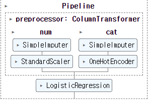
전처리와 학습까지 완성된 파이프라인의 모습입니다.

점수측정

input

print(clf.score(X_train,y_train))
print(clf.score(X_test,y_test))

output

0.76625
0.775

최적화

input

from sklearn.model_selection import GridSearchCV 
# 최적의 하이퍼파라미터 선택을 위한 작업
# 파이프라인의step__파라미터
param_grid={
    'preprocessor__num__imputer__strategy': ['mean', 'median'],
    'classifier__C': [0.0001, 0.001, 0.01, 0.1, 1.0, 10, 100]
}
grid_search=GridSearchCV(clf, param_grid, cv=10) # cv 교차검증 횟수
grid_search.fit(X,y)

output

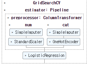
파라미터를 얼마나 주어야하는지 알아보기위해 GridSearch를 이용하여 검사해줍니다.

파라미터 조합

input

#파라미터 조합
grid_search.cv_results_['params']

output

[{'classifierC': 0.0001, 'preprocessornumimputerstrategy': 'mean'},
{'classifierC': 0.0001, 'preprocessornumimputerstrategy': 'median'},
{'classifierC': 0.001, 'preprocessornumimputerstrategy': 'mean'},
{'classifierC': 0.001, 'preprocessornumimputerstrategy': 'median'},
{'classifierC': 0.01, 'preprocessornumimputerstrategy': 'mean'},
{'classifierC': 0.01, 'preprocessornumimputerstrategy': 'median'},
{'classifierC': 0.1, 'preprocessornumimputerstrategy': 'mean'},
{'classifierC': 0.1, 'preprocessornumimputerstrategy': 'median'},
{'classifierC': 1.0, 'preprocessornumimputerstrategy': 'mean'},
{'classifierC': 1.0, 'preprocessornumimputerstrategy': 'median'},
{'classifierC': 10, 'preprocessornumimputerstrategy': 'mean'},
{'classifierC': 10, 'preprocessornumimputerstrategy': 'median'},
{'classifierC': 100, 'preprocessornumimputerstrategy': 'mean'},
{'classifierC': 100, 'preprocessornumimputerstrategy': 'median'}]

정확도 측정

input

#검증용 데이터셋의 정확도 
scores=grid_search.cv_results_['mean_test_score']
scores

output

array([0.727, 0.728, 0.748, 0.748, 0.75 , 0.75 , 0.754, 0.75 , 0.754,
0.753, 0.754, 0.753, 0.754, 0.753])

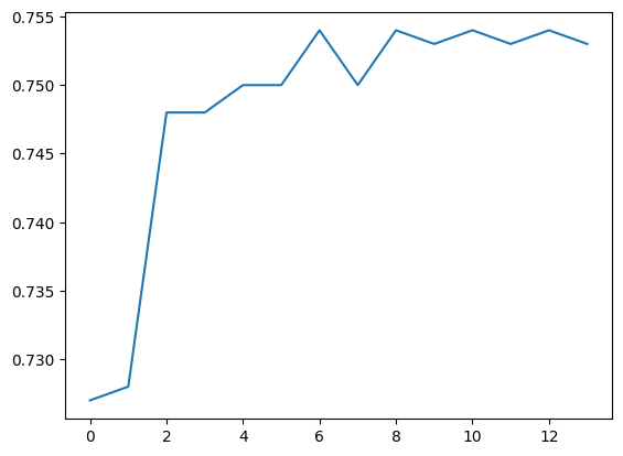
결과가 드라마틱하게 바뀌지는 않습니다.

최적화 점수

input

import matplotlib.pyplot as plt 
print(max(scores)) #최고점수
plt.plot(scores)

output

0.7540000000000001
[<matplotlib.lines.Line2D at 0x1ee37bf9850>]

결과

input

print(grid_search.best_score_) #최고점수
print(grid_search.best_params_) #최적의 파라미터

output

0.7540000000000001
{'classifierC': 0.1, 'preprocessornumimputerstrategy': 'mean'}

오늘은 파이프라인을 통해 데이터 전처리와 학습을 자동화 시키는 방법과 그리드서치를 이용하여 최적의 파라미터 값을 찾아내는 방법을 배워보았습니다. 결과값이 예상과는 다르게 나왔지만, 방법을 알아가는게 중요하다고 생각합니다 😂

😁 power through to the end 😁

Jayce_97

AI (ML/DL) 학습

이전 포스트

Python 전처리 자동화