시작하며
올해 상반기 부스트캠프 AI TECH 활동을 하며 같은 팀원분들과 함께 매주 논문 리뷰를 진행했었다.
부캠 활동이 끝난 뒤에도 논문 리뷰를 이어갔는데 정리와 기록의 필요성을 느껴 지난 논문 리뷰 몇개와 앞으로의 논문 리뷰는 블로그에도 기록하고자 한다.
첫 게시글은 'Efficient Estimation of Word Representations in Vector Space'(word2vec)으로 정했다. 제목에서도 볼 수 있듯 'Efficient'와 'Vector'가 핵심 키워드라고 볼 수 있다. 이 논문은 벡터를 이용한 단어 표현과 계산 복잡도 측면에서의 효율성을 골자로 한다.
(설명이 부족한 부분이나 잘못된 정보가 있을 수 있습니다. 댓글로 알려주시면 확인 후 수정하도록 하겠습니다.)
Efficient Estimation of Word Representations in Vector Space
1 Introduction
Many current NLP systems and techniques treat words as atomic units - there is no notion of similarity between words, as these are represented as indices in a vocabulary.
어떠한 단어를 표현할 때 vocab의 index로 표현하는 방식으로는 단어 간 유사성을 파악할 수 없다. (거기다 vocab이 커질수록 one-hot vector의 차원이 커지게 된다.)
With progress of machine learning techniques in recent years, it has become possible to train more complex models on much larger data set, and they typically outperform the simple models. Probably the most successful concept is to use distributed representations of words [10]. For example, neural network based language models significantly outperform N-gram models [1, 27, 17].
더 거대한 데이터셋에서 복잡한 모델을 훈련하는 것이 가능해졌고 또 그러한 모델이 단순한 모델보다 더 좋은 성능을 보인다. 예를 들어 N-gram model보다 language model 기반의 신경망이 더 좋은 성능을 보인다.
1.1 Goal of Paper
The main goal of this paper is to introduce techniques that can be used for learning high-quality word vectors from huge data sets with billions of words, and with millions of words in the vocabulary.
(...)
We use recently proposed techniques for measuring the quality of the resulting vector representations, with the expectation that not only will similar words tend to be close to each other, but that words can have multiple degrees of similarity [20].
(...)
Somewhat surprisingly, it was found that similarity of word representations goes beyond simple syntactic regularities. Using a word offset technique where simple algebraic operations are performed on the word vectors, it was shown for example that vector(”King”) - vector(”Man”) + vector(”Woman”) results in a vector that is closest to the vector representation of the word Queen [20].
고품질의 word vector를 훈련시키는 것이 목적이다. 또 단순히 유사한 단어들이 벡터 공간 상에서 가까이 있도록 하는 것뿐만 아니라 다양한 유사도를 반영할 수 있도록 하는 것이 목적이다.
vector('King') - vector('Man') - vector('Woman') = vector('Queen') 과 같은 연산은 다양한 유사도를 정확히 반영했기 때문에 가능하지 않을까 하는 생각이 든다.
1.2 Previous Work
A very popular model architecture for estimating neural network language model (NNLM) was proposed in [1], where a feedforward neural network with a linear projection layer and a non-linear hidden layer was used to learn jointly the word vector representation and a statistical language model.
이 논문에서는 언어학적으로 정확한 의미 반영과 높은 효율성을 갖는 모델을 찾기 위해 이전의 NNLM과 CBOW model, Skip-gram model을 비교한다.
2 Model Architectures
Similar to [18], to compare different model architectures we define first the computational complexity of a model as the number of parameters that need to be accessed to fully train the model. Next, we will try to maximize the accuracy, while minimizing the computational complexity.
For all the following models, the training complexity is proportional to
O = E × T × Q, (1)
where E is number of the training epochs, T is the number of the words in the training set and Q is defined further for each model architecture. Common choice is E = 3 − 50 and T up to one billion. All models are trained using stochastic gradient descent and backpropagation [26].
서로 다른 모델 아키텍쳐를 비교하기 위해 computational complexity를 모델을 train할 때 access되는 파라미터의 개수를 이용해 정의한다. 또한 비교를 통해 정확성은 높이고 연산 복잡도는 줄이고자 한다.
좀 더 자세히 training complexity(O)는 training epochs(E), number of the words(T), model architecture(Q)에 비례한다. 대개 epochs은 3에서 50이며 T는 최대 10억여개에 달한다.
2.1 Feedforward Neural Net Language Model(NNLM)
The probabilistic feedforward neural network language model has been proposed in [1]. It consists of input, projection, hidden and output layers. At the input layer, N previous words are encoded using 1-of-V coding, where V is size of the vocabulary. The input layer is then projected to a projection layer P that has dimensionality N × D, using a shared projection matrix.
(...)
Thus, the computational complexity per each training example is
Q = N × D + N × D × H + H × V, (2)
where the dominating term is H × V . However, several practical solutions were proposed for avoiding it; either using hierarchical versions of the softmax [25, 23, 18], or avoiding normalized models completely by using models that are not normalized during training [4, 9]. With binary tree representations of the vocabulary, the number of output units that need to be evaluated can go down to around log2(V ). Thus, most of the complexity is caused by the term N × D × H.
쉽게 말해 N개의 맥락 단어를 통해 1개의 타겟 단어를 예측하는 방식으로 훈련된다. 각 단어는 input layer, projection layer, output layer를 통해 타겟 단어의 확률 점수로 변환되고 이를 통해 최종적으로 타겟 단어를 예측할 수 있다.
각 layer에서의 변환을 좀 더 자세히 들여다보면 다음과 같다.
먼저 각 단어는 V차원(vocabulary)을 갖는 one-hot vector로 표현된다. 그 후 shared projection matrix (V,D)를 통해 각 one-hot vector는 D차원의 dense vector로 변환된다.
이 후 N개의 dense vector는 concat되어 NxD 차원을 갖는 projection layer가 되고 hidden matrix ((NxD),H)를 통해 1xH 차원의 hidden layer로 변환된다.
hidden layer는 다시 (H,V) matrix와의 연산을 통해 1xV 벡터로 변환되고 softmax function을 통해 vocab 속 각 단어에 대한 확률점수로 변환된다. softmax 후 최댓값을 구하는 것은 결국 vocab에 대해 one-hot vector를 구하는 것과 같다.
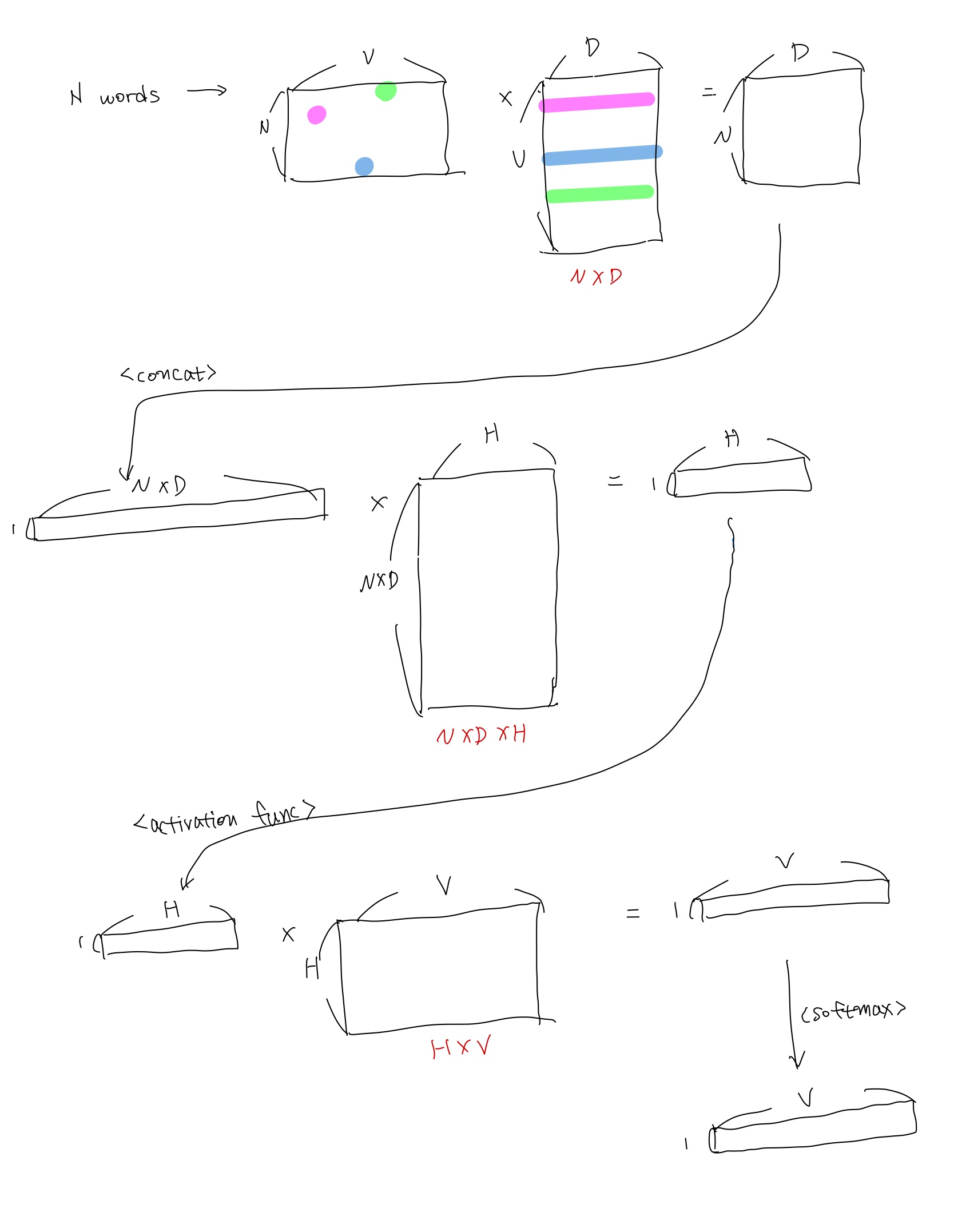
빨간 글씨로 access된 파라미터의 수를 표시하였다.
N개의 one-hot vector와 shared projection matrix 간의 행렬곱은 곧 shared projection matrix에서 one-hot vector의 index를 따라 최대 N개의 행을 선택하는 것과 같다. 즉 shared projection matrix의 전체 파라미터 수는 VxD이지만 훈련 시 실제 access되는 파라미터의 수는 NxD라는 것.
때문에 NNLM의 모델 아키텍처 상 계산 복잡도 Q는
NxD + NxDxH + HxV 와 같다.
이 중 HxV의 영향이 가장 큰데 이는 hierarchical softmax를 통해 Hx(logV)로 줄일 수 있다.(log의 밑은 2인데 편의상 'log'로 표현하겠다) 이렇게 할 경우 가장 지배적인 영향력을 가지는 항은 NxDxH가 된다. 지배적인 항을 파악하는 것은 추후 모델 별 계산 복잡도를 비교할 때 도움을 준다.
2.2 Reccurent Neural Net Language Model(RNNLM)
The RNN model does not have a projection layer; only input, hidden and output layer. What is special for this type of model is the recurrent matrix that connects hidden layer to itself, using time-delayed connections.
(...)
The complexity per training example of the RNN model is
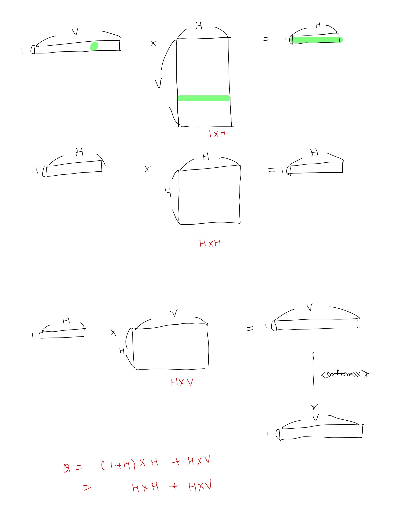
Q = H × H + H × V, (3)
where the word representations D have the same dimensionality as the hidden layer H. Again, the term H × V can be efficiently reduced to H × log2(V ) by using hierarchical softmax. Most of the complexity then comes from H × H.
RNN을 이용해 학습을 수행한다. projection layer 없이 input, hidden, output만으로 구성된다. hidden layer는 reccurent matrix를 통해 곧 자기자신의 hidden layer와 연결된다.
Q = HxH + HxV로 정리되고 HxV가 지배적인 항이지만 위와 마찬가지로 Hx(logV)가 되어 HxH가 지배적인 항이 된다.
3 New Log-linear Models
3.1 Continuous Bag-of-Words Model(CBOW)
The first proposed architecture is similar to the feedforward NNLM, where the non-linear hidden layer is removed and the projection layer is shared for all words (not just the projection matrix); thus, all words get projected into the same position (their vectors are averaged). We call this architecture a bag-of-words model as the order of words in the history does not influence the projection. Furthermore, we also use words from the future; we have obtained the best performance on the task introduced in the next section by building a log-linear classifier with four future and four history words at the input, where the training criterion is to correctly classify the current (middle) word. Training complexity is then
Q = N × D + D × log2(V ). (4)
We denote this model further as CBOW, as unlike standard bag-of-words model, it uses continuous distributed representation of the context.
NNLM과의 주요한 차이점은 projection 방식과 non-linear hidden layer의 부재이다.
우선 dense vector로 표현된 N개의 단어에 대해 average를 구하고 이를 V차원으로 변환한다. 단순 평균을 내기 때문에 단어의 순서는 의미가 없어진다.
한가지 유의할 점은 타겟 단어 예측을 위한 맥락 단어의 선별이 단순히 과거 시점에서만 이뤄지는 것이 아니라 미래 시점에서도 이루어진다는 것이다. 쉽게 말해 단어 sequence가 있을 때 앞뒤 단어들을 통해 가운데 단어를 예측한다.
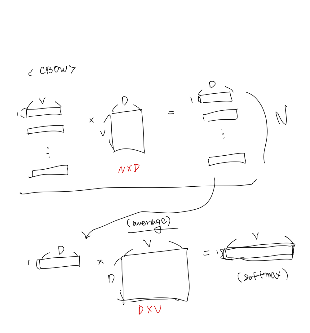
Q = NxD + DxV -> NxD + Dx(logV)
3.2 Continuous Skip-gram Model
The second architecture is similar to CBOW, but instead of predicting the current word based on the context, it tries to maximize classification of a word based on another word in the same sentence. More precisely, we use each current word as an input to a log-linear classifier with continuous projection layer, and predict words within a certain range before and after the current word.
(...)
The training complexity of this architecture is proportional to
Q = C × (D + D × log2(V )), (5)
where C is the maximum distance of the words. Thus, if we choose C = 5, for each training word we will select randomly a number R in range < 1; C >, and then use R words from history and R words from the future of the current word as correct labels. This will require us to do R × 2 word classifications, with the current word as input, and each of the R + R words as output.
Skip-gram은 CBOW와 반대라고 생각하면 될 것 같다. 주변 맥락 단어로 타겟 단어를 예측하는 것이 아니라 어떤 한 단어를 이용해 앞뒤 R개의 단어를 예측하는 방식이다. 이때 R은 1 이상 C 이하의 범위를 가진다.
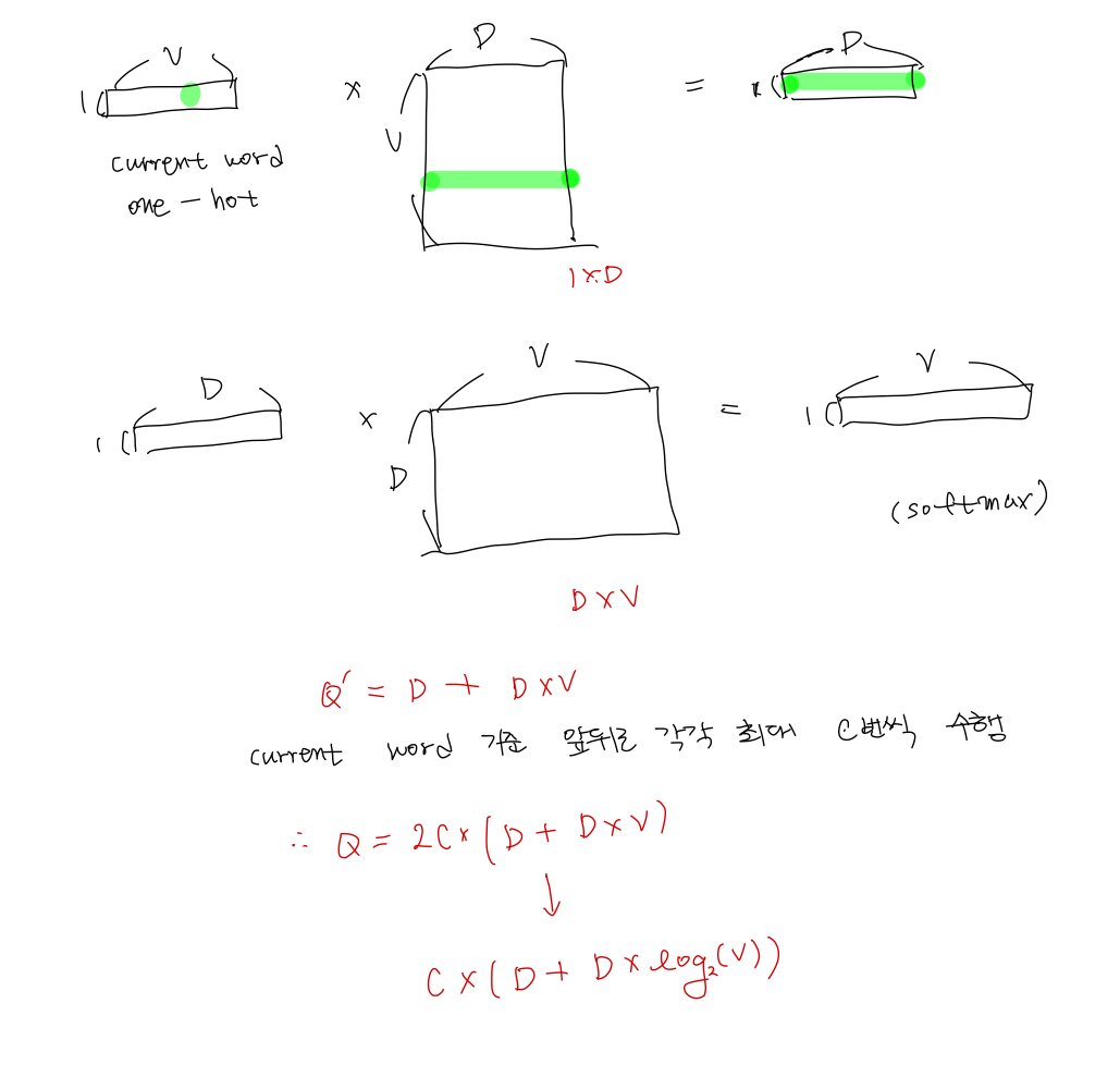
Q = C x (D + DxlogV)
4 Result
Although it is easy to show that word France is similar to Italy and perhaps some other countries, it is much more challenging when subjecting those vectors in a more complex similarity task, as follows. We follow previous observation that there can be many different types of similarities between words, for example, word big is similar to bigger in the same sense that small is similar to smaller. Example of another type of relationship can be word pairs big - biggest and small - smallest [20]. We further denote two pairs of words with the same relationship as a question, as we can ask: ”What is the word that is similar to small in the same sense as biggest is similar to big?”
어떤 단어에 대해 단순히 '가장 유사한 단어'를 찾아내는 것뿐만 아니라 다양한 유사도를 반영하는 것이 필요하다.
단어 'big'에 대해서 'small-smallest'과 같은 관계를 갖는 단어를 찾아내는 것은 인공지능 모델이 실제로 사람처럼 언어를 다루는 데에 필수적인 기능이라 할 수 있기 때문이다.
Somewhat surprisingly, these questions can be answered by performing simple algebraic operations with the vector representation of words. To find a word that is similar to small in the same sense as biggest is similar to big, we can simply compute vector X = vector(”biggest”) − vector(”big”) + vector(”small”). Then, we search in the vector space for the word closest to X measured by cosine distance, and use it as the answer to the question (we discard the input question words during this search). When the word vectors are well trained, it is possible to find the correct answer (word smallest) using this method.
위와 같은 작업은 단순히 word vector 간의 algebraic operation으로 수행될 수 있다. 벡터값을 이용해 계산한 후 벡터 공간 상에서 계산 결과 벡터와 가장 가까이 있는 word vector를 선택하면 된다.
Finally, we found that when we train high dimensional word vectors on a large amount of data, the resulting vectors can be used to answer very subtle semantic relationships between words, such as a city and the country it belongs to, e.g. France is to Paris as Germany is to Berlin.
big-biggest의 예처럼 syntatic task 외에도 semantic task도 잘 수행할 수 있다.
4.1 Task Description
To measure quality of the word vectors, we define a comprehensive test set that contains five types of semantic questions, and nine types of syntactic questions.
word vector의 퀄리티를 측정하기 위해서 5종류의 semantic question과 9종류의 syntactic question을 이용해 test set을 구성했다.
4.2 Maximization of Accuracy
word vectors를 훈련시키기 위해 'Google News corpus'를 사용했다고 한다. 해당 corpus는 60억개의 토큰을 포함하고 있으며 논문 저자들은 vocab size를 가장 빈도수가 높은 백만개의 단어로 제한했다고 한다.
짧은 시간 안에 효과적으로 다양한 모델 아키텍쳐를 실험하기 위해 경우데 따라 vocab을 3만개 단어로 제한하는 등의 기법을 사용했으며, 단일 모델(CBOW)을 사용하면서 word vector dimensionality나 training words를 변경하는 실험도 했다고 한다.
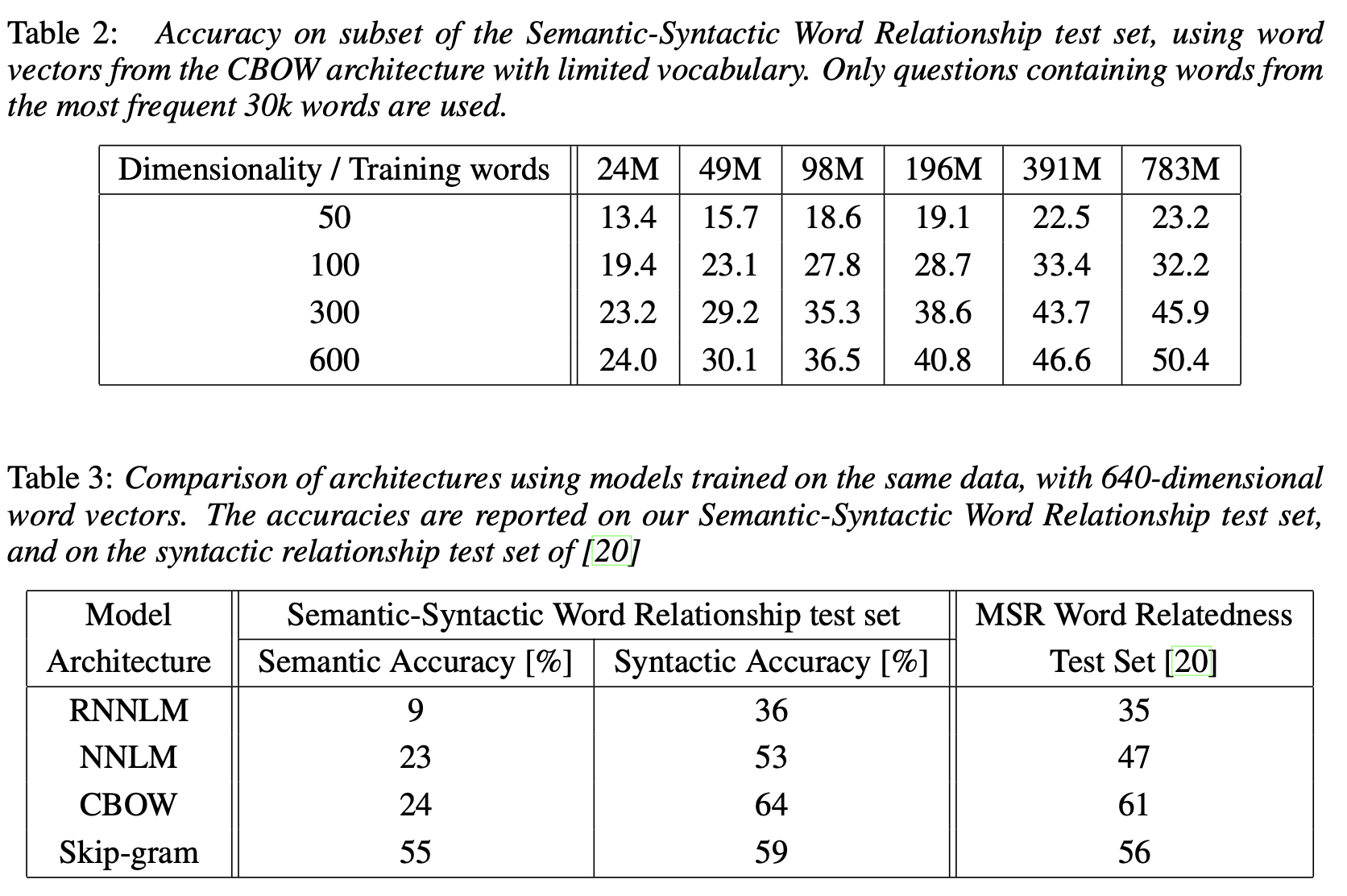
- 일반적으로는 word vector dimensionality와 training words를 늘릴수록 accuracy가 상승하지만, 일정 수준 이상의 증가는 의미가 없는 것으로 나타났다.
구체적으로는 dim을 제한하고 training words만 늘릴 경우 일정 수준 이상으로는 accuracy가 더이상 증가하지 않았고 반대의 경우도 마찬가지였다.
표현해야 하는 단어의 수를 training words, 표현력을 dim이라고 볼 경우 '표현력이 제한되어 있을 경우 일정 개수 이상의 단어를 표현할 수 없고', '표현할 단어의 개수가 제한되어 있을 경우 더 높은 표현력을 갖는게 의미가 없다'는 식으로 이해하면 될 것 같다. - 모델의 경우는 CBOW, Skip-gram이 높은 정확도를 보였다. semantic, syntactic 모두에서 높은 성능을 보인 모델은 Skip-gram이라고 할 수 있다.
4.3 Comparison of Model Architectures
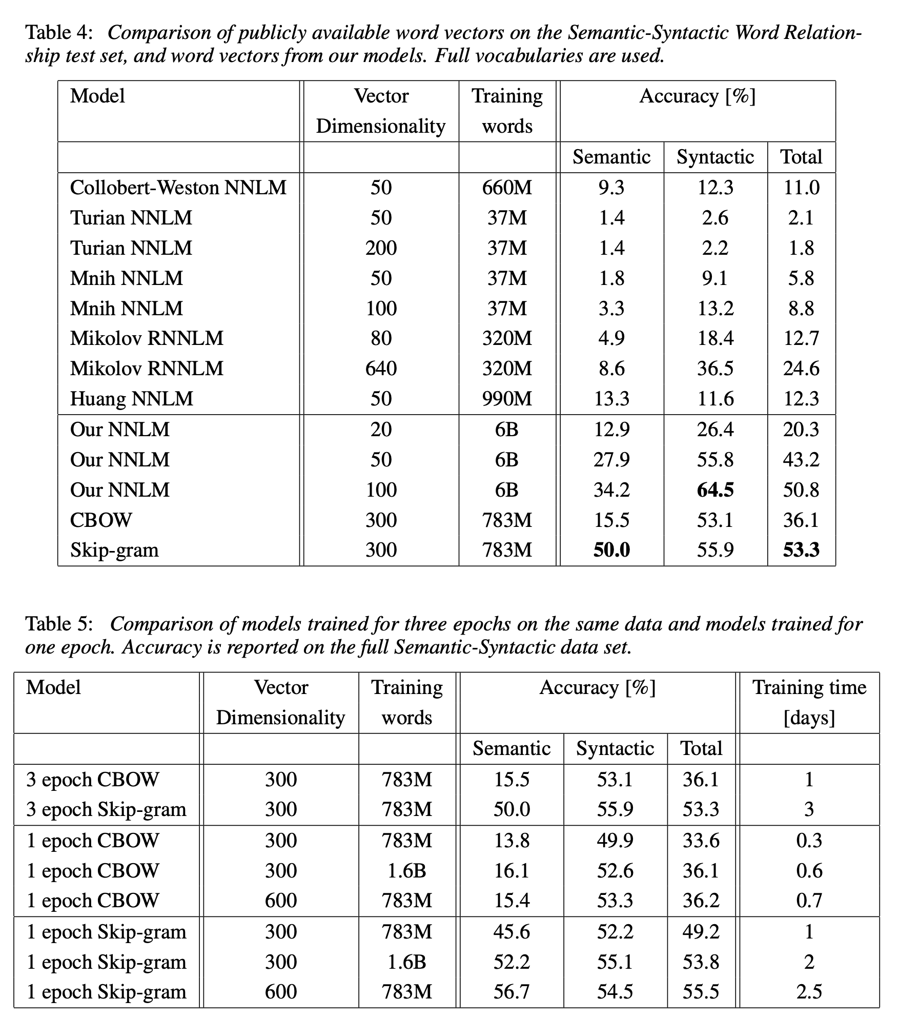
대체로 Skip-gram이 semantic, syntactic test set 모두에서 준수한 성능을 보인다. 다만 한가지 단점이라면 다른 모델에 비해 계산 복잡도가 높아서 훈련시간이 조금 더 소요된다.
4.4 Large Scale Parallel Training of Models
4.5 Microsoft Research Sentence Completion Challenge
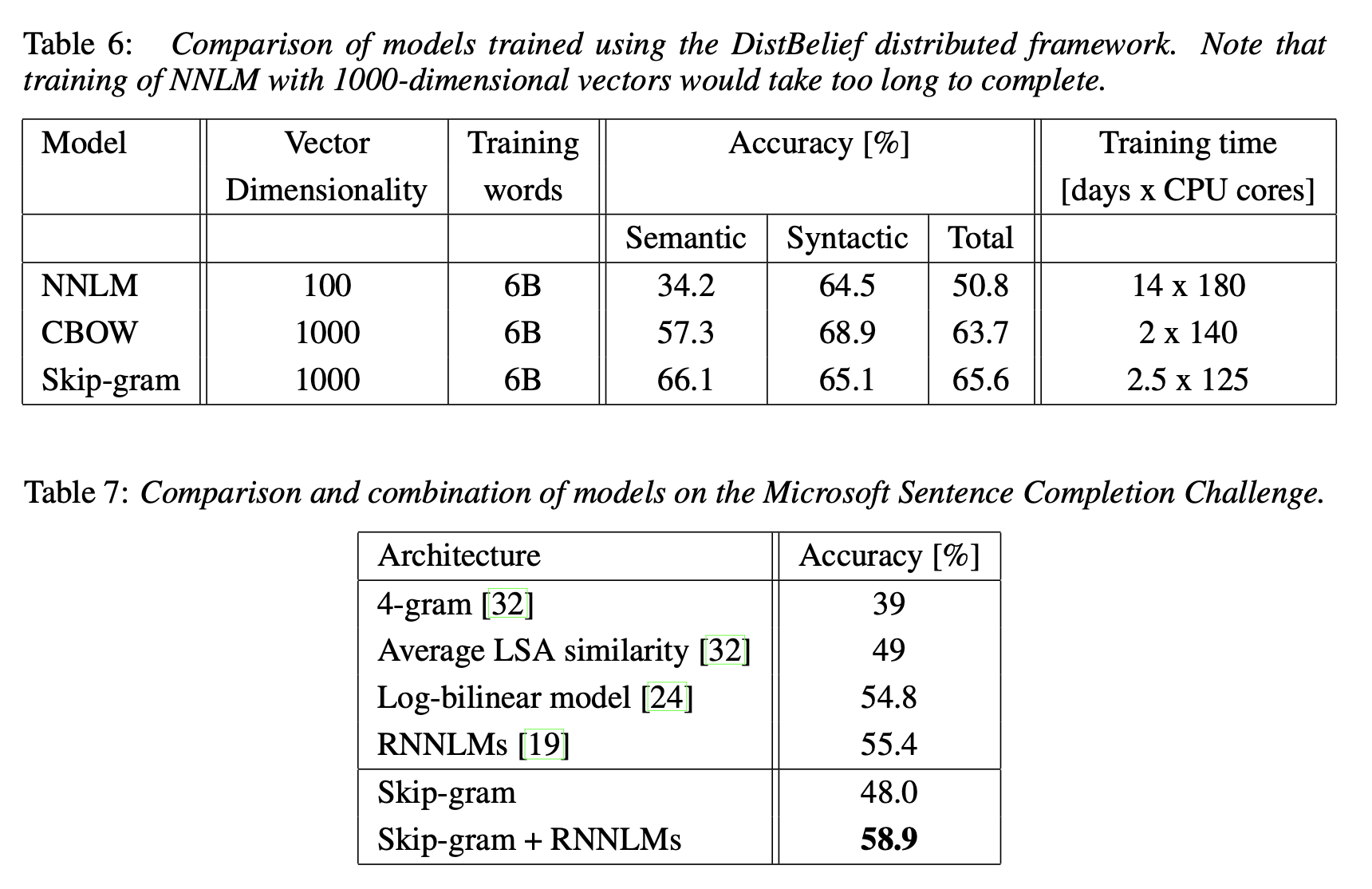
유사한 결과가 나타난다.
Microsoft Sentence Completion Challenge(5지선다형)에 대해선 Skip-gram 단독으로는 Accuracy가 다소 떨어지는 모습을 보였지만 Skip-gram + RNNLMs 조합으로는 가장 높은 정확도를 보였다.
5 Examples of the Learned Relationships
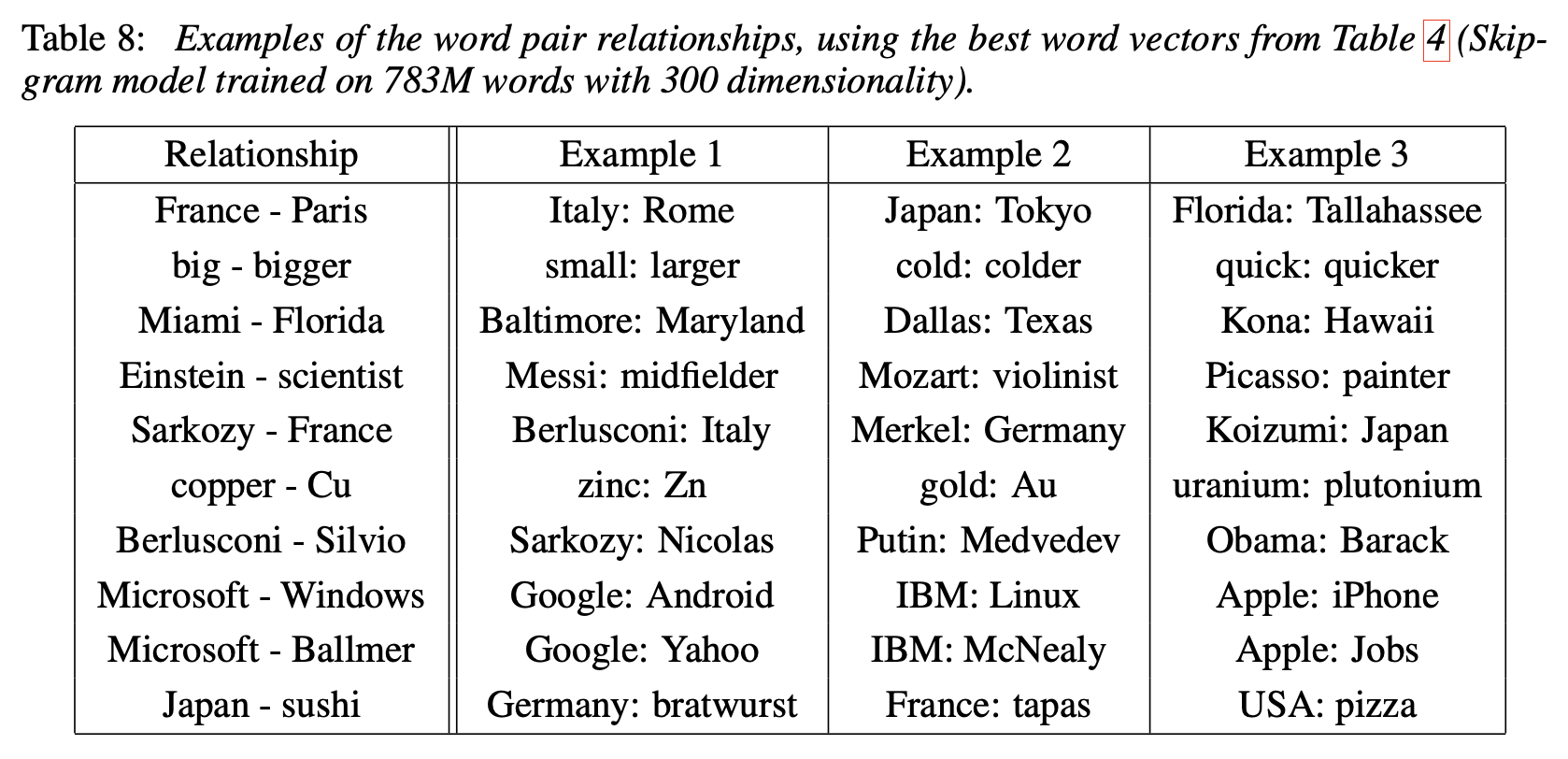
위의 실험에서 가장 성능이 좋았던 모델(Skip-gram on 783M words with 300 dim)의 word vectors를 이용해서 위에서 언급한 algebraic operation을 수행한 결과 예시이다.
syntactic task뿐만 아니라 semantic task도 잘 수행하는 것을 볼 수 있다.
6 Conclusion
We observed that it is possible to train high quality word vectors using very simple model architectures, compared to the popular neural network models (both feedforward and recurrent). Because of the much lower computational complexity, it is possible to compute very accurate high dimensional word vectors from a much larger data set.
(...)
The neural network based word vectors were previously applied to many other NLP tasks, for example sentiment analysis [12] and paraphrase detection [28]. It can be expected that these applications can benefit from the model architectures described in this pape
(...)
We believe that our comprehensive test set will help the research community to improve the existing techniques for estimating the word vectors. We also expect that high quality word vectors will become an important building block for future NLP applications.
제목에서부터 언급되었듯 효율적이고 정확한 word vector의 훈련에 대해 연구한 논문이라고 볼 수 있다. 적은 계산 복잡도로 정확한 high dimensional word vectors를 훈련할 수 있음을 보였다.
다양한 NLP task에 적용되는 word vector들에도 도움을 줄 수 있고 나아가 NLP application의 주요한 building block이 될 수 있다고 믿는다고 한다.
마치며
배울 점이 많은 논문이었다. 단어쌍의 semantic, syntactic한 부분을 모두 고려하고자 했으며 효율성에 대해 고민하고 개선한 부분이 인상적이었다.
축적된 data 양의 폭발적 증대와 하드웨어 성능의 향상은 인공지능 분야의 엄청난 발전을 가져오긴 했지만 반대로 말하면 그만한 자원을 확보하지 않을 경우에 연구나 적용이 어려워진다는 것을 의미하기도 했다. 계산 복잡도 측면에서의 효율성을 연구하는 것은 반드시 필요한 일이었다고 생각한다.
어느정도 개념은 잡았지만 아직도 부족한 점이 있다고 느낀다. 모델 구조와 계산 복잡도 부분에서 조금 모호한 부분이 남아있다. word2vec은 NLP 분야에서 일종의 근간이 되는 논문인만큼 간단히 구현해보면서 더 이해해보도록 해야겠다.
References