안녕하세요. Gameeye에서 deeplol.gg 서비스를 개발 중인 김철기입니다.
클라우드 서버 인프라 구축, 백엔드 개발, 딥러닝 모델 연구를 담당하고 있습니다.
해당 포스팅은 Style Transfer Model 서비스 해보기 시리즈에서 사용한 Style Transfer Model 코드를 리뷰하는 포스팅입니다. 시리즈에서는 Tensorflow Hub에서 받아온 Model을 바로 사용하여 Model의 이해없이도 서비스를 구성하는데에는 문제가 없으나 양심상 사용한 Model의 이해는 필요하다고 생각되어 리뷰하게 되었습니다.
2015년에 Leon A. Gatys, Alexander S. Ecker, Matthias Bethge가 작성한 논문 "A Neural Algorithm of Artistic Style"을 기반으로 작성된 코드입니다. 꽤나 오래된 논문이고 기술이지만 개인적으로 자연어와 시계열 기반 데이터와 Model을 주로 다뤄왔던 저에게는 흥미로운 시간이었습니다.
시작하기에 앞서..
해당 포스팅은 기본적으로 Python, Tensorflow, 선형대수의 이해가 있다는 가정하에 작성되었습니다.
참고 자료
결과 예시
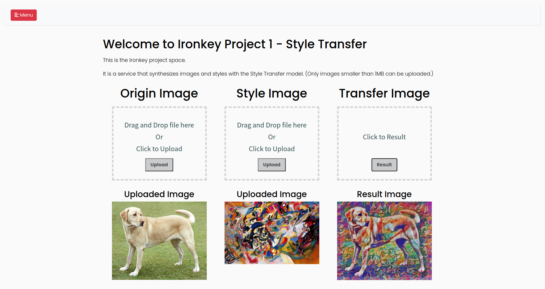
구현한 서비스에서 출력한 예시입니다. 원본 이미지인 강아지 이미지와 스타일 이미지인 칸딘스키 7번 작품을 입력으로 넣으면 강아지 이미지에 스타일 이미지의 스타일이 합성된 이미지가 결과물로 출력됩니다.
코드 리뷰
Tensorflow Hub 모듈을 이용하는 방법
Tensorflow Hub의 모듈을 이용하면 빠르게 우리가 원하는 결과를 출력해볼 수 있습니다. 구현했던 서비스는 해당 모듈을 이용했습니다.
테스트에 필요한 이미지를 로드합니다.
content_path = tf.keras.utils.get_file('YellowLabradorLooking_new.jpg', 'https://storage.googleapis.com/download.tensorflow.org/example_images/YellowLabradorLooking_new.jpg')

style_path = tf.keras.utils.get_file('kandinsky5.jpg','https://storage.googleapis.com/download.tensorflow.org/example_images/Vassily_Kandinsky%2C_1913_-_Composition_7.jpg')

def load_img(path_to_img):
  max_dim = 512
  img = tf.io.read_file(path_to_img)
  img = tf.image.decode_image(img, channels=3)
  img = tf.image.convert_image_dtype(img, tf.float32)

  shape = tf.cast(tf.shape(img)[:-1], tf.float32)
  long_dim = max(shape)
  scale = max_dim / long_dim

  new_shape = tf.cast(shape * scale, tf.int32)

  img = tf.image.resize(img, new_shape)
  img = img[tf.newaxis, :]
  return img

content_image = load_img(content_path)
style_image = load_img(style_path)
Tensorflow Hub에서 모듈을 가져와 출력을 확인합니다.
def tensor_to_image(tensor):
  tensor = tensor*255
  tensor = np.array(tensor, dtype=np.uint8)
  if np.ndim(tensor)>3:
    assert tensor.shape[0] == 1
    tensor = tensor[0]
  return PIL.Image.fromarray(tensor)

import tensorflow_hub as hub
hub_module = hub.load('https://tfhub.dev/google/magenta/arbitrary-image-stylization-v1-256/1')
stylized_image = hub_module(tf.constant(content_image), tf.constant(style_image))[0]
tensor_to_image(stylized_image)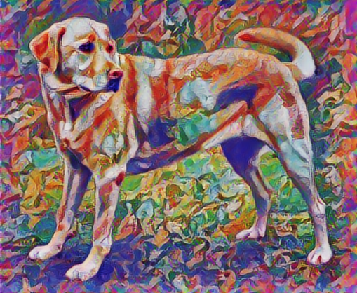
VGG19 모델을 이용해 직접 구현하기
VGG19 모델은 Convolution Neural Network로 구성된 이미지 분류 모델입니다. 해당 모델은 이미지를 분류하기 위해 각 Convolution 층에서 이미지의 특성을 추출합니다. 우리는 모델의 이런 특성을 활용하여 이미지 콘텐츠와 스타일 특성을 정의할 수 있습니다.
include_top=False으로 설정된 아래 코드로 마지막 분류 단계가 누락된 VGG19 모델을 불러올 수 있습니다.
vgg = tf.keras.applications.VGG19(include_top=False, weights='imagenet')콘텐츠 특성과 스타일 특성을 정의합니다.
앞서 설명드린 것처럼 이미지 분류 모델은 이미지의 특성을 추출하는 작업이 포함되어있습니다. 따라서 모델의 중간층에 접근하여 이미지의 콘텐츠와 스타일을 추출할 수 있습니다.
content_layers = ['block5_conv2']

style_layers = ['block1_conv1',
                'block2_conv1',
                'block3_conv1',
                'block4_conv1',
                'block5_conv1']

num_content_layers = len(content_layers)
num_style_layers = len(style_layers)
입력받은 layer_names list에 해당하는 중간층의 출력값을 반환하는 모델입니다.
def vgg_layers(layer_names):
""" 중간층의 출력값을 배열로 반환하는 vgg 모델을 만듭니다."""
# 이미지넷 데이터셋에 사전학습된 VGG 모델을 불러옵니다
vgg = tf.keras.applications.VGG19(include_top=False, weights='imagenet')
vgg.trainable = False
outputs = [vgg.get_layer(name).output for name in layer_names]
model = tf.keras.Model([vgg.input], outputs)
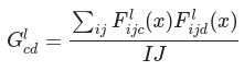
return modelStyle Transfer에서는 feature map의 correlation을 더욱 효율적으로 표현하기 위해 Gram Matrix를 사용합니다. 수식은 아래와 같습니다.
def gram_matrix(input_tensor):
  result = tf.linalg.einsum('bijc,bijd->bcd', input_tensor, input_tensor)
  input_shape = tf.shape(input_tensor)
  num_locations = tf.cast(input_shape[1]*input_shape[2], tf.float32)
  return result/(num_locations)
정의한 style layers와 content layers의 텐서를 반환하는 모델입니다. style 텐서의 경우 앞서 정의한 gram_matrix가 적용됩니다.
class StyleContentModel(tf.keras.models.Model):
  def __init__(self, style_layers, content_layers):
    super(StyleContentModel, self).__init__()
    self.vgg =  vgg_layers(style_layers + content_layers)
    self.style_layers = style_layers
    self.content_layers = content_layers
    self.num_style_layers = len(style_layers)
    self.vgg.trainable = False

  def call(self, inputs):
    "[0,1] 사이의 실수 값을 입력으로 받습니다"
    inputs = inputs*255.0
    preprocessed_input = tf.keras.applications.vgg19.preprocess_input(inputs)
    outputs = self.vgg(preprocessed_input)
    style_outputs, content_outputs = (outputs[:self.num_style_layers],
                                      outputs[self.num_style_layers:])

    style_outputs = [gram_matrix(style_output)
                     for style_output in style_outputs]

    content_dict = {content_name:value
                    for content_name, value
                    in zip(self.content_layers, content_outputs)}

    style_dict = {style_name:value
                  for style_name, value
                  in zip(self.style_layers, style_outputs)}

    return {'content':content_dict, 'style':style_dict}
style과 content 텐서를 추출할 수 있으니 추출된 값을 기반으로 전이 알고리즘을 구현합니다. loss를 계산하는데 사용되는 target은 style 이미지에서 추출한 style 텐서와 content 이미지에서 추출한 content 텐서가 됩니다. 우리는 입력 이미지의 style 텐서가 style target 텐서와 가까우면서 content 이미지의 content 텐서가 여전히 content target 텐서와 가깝게 학습합니다.
target을 정의합니다.
style_targets = extractor(style_image)['style']
content_targets = extractor(content_image)['content']
최적화시킬 이미지를 정의합니다.
image = tf.Variable(content_image)픽셀 값을 0~1 사이 값으로 클리핑하는 함수입니다.
def clip_0_1(image):
  return tf.clip_by_value(image, clip_value_min=0.0, clip_value_max=1.0)
옵티마이저를 정의합니다.
opt = tf.optimizers.Adam(learning_rate=0.02, beta_1=0.99, epsilon=1e-1)최적화를 시키기 위해 loss를 계산하는 방법을 정의합니다. 위에서 정의한 것처럼 입력 이미지의 style 텐서가 style target 텐서와 가까우면서 content 이미지의 content 텐서가 여전히 content target 텐서와 가깝게 학습되도록 loss를 정의합니다. style 오차의 가중합과 콘텐츠 오차의 가중합을 각각 정의하고 더해주는데 각 가중합에 사용자가 정의한 가중치(style_weight, content_weight)를 곱해줍니다. 곱해지는 가중치를 수정하는 것으로 style과 content가 최적화에 영향을 주는 정도를 조절할 수 있습니다.
style_weight=1e-2
content_weight=1e4
def style_content_loss(outputs):
    style_outputs = outputs['style']
    content_outputs = outputs['content']
    style_loss = tf.add_n([tf.reduce_mean((style_outputs[name]-style_targets[name])**2)
                           for name in style_outputs.keys()])
    style_loss *= style_weight / num_style_layers

    content_loss = tf.add_n([tf.reduce_mean((content_outputs[name]-content_targets[name])**2)
                             for name in content_outputs.keys()])
    content_loss *= content_weight / num_content_layers
    loss = style_loss + content_loss
    return loss
계산된 loss를 기반으로 모델과 이미지를 업데이트 시킵니다.
@tf.function()
def train_step(image):
  with tf.GradientTape() as tape:
    outputs = extractor(image)
    loss = style_content_loss(outputs)

  grad = tape.gradient(loss, image)
  opt.apply_gradients([(grad, image)])
  image.assign(clip_0_1(image))

import time
start = time.time()

epochs = 3
steps_per_epoch = 100

step = 0
for n in range(epochs):
  for m in range(steps_per_epoch):
    step += 1
    train_step(image)
    print(".", end='')
  display.clear_output(wait=True)
  display.display(tensor_to_image(image))
  print("훈련 스텝: {}".format(step))

end = time.time()
print("전체 소요 시간: {:.1f}".format(end-start))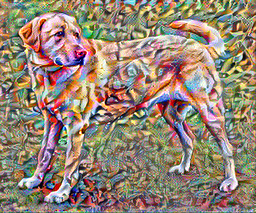
지금까지 구현한 코드로도 충분한 결과를 얻었다고 생각할 수 있습니다. 하지만 현 방식의 단점으로 high frequency artifact가 생겨나는 부분이있습니다. 우리는 high frequency artifact 요소또한 loss를 계산하는 수식에 포함시켜 regularization 해줄 수 있습니다.
high frequency artifact를 계산하는 함수입니다.
def high_pass_x_y(image):
  x_var = image[:,:,1:,:] - image[:,:,:-1,:]
  y_var = image[:,1:,:,:] - image[:,:-1,:,:]

  return x_var, y_var
reqularization 항의 가중치를 정의하고 train_step 함수를 수정해줍니다. 기존 loss 계산식에 가중치가 곱해진 reqularization항이 추가로 더해집니다. optimizer는 loss가 작아지도록 학습하기 때문에 high frequency artifact가 작은 결과에 도달하게 합니다.
total_variation_weight=30
@tf.function()
def train_step(image):
  with tf.GradientTape() as tape:
    outputs = extractor(image)
    loss = style_content_loss(outputs)
    loss += total_variation_weight*tf.image.total_variation(image)

  grad = tape.gradient(loss, image)
  opt.apply_gradients([(grad, image)])
  image.assign(clip_0_1(image))
마지막으로 수정된 loss 계산식이 적용된 최적화를 진행합니다.
epochs = 10
steps_per_epoch = 100

step = 0
for n in range(epochs):
  for m in range(steps_per_epoch):
    step += 1
    train_step(image)
    print(".", end='')
  display.clear_output(wait=True)
  display.display(tensor_to_image(image))
  print("훈련 스텝: {}".format(step))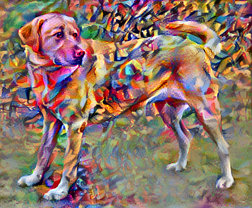
정리
논문과 colab 코드를 바탕으로 이해한 내용을 잘 정리해보고 싶었는데 이미 워낙 정리가 잘 되어있는 코드여서 제 포스팅이 크게 도움이 될지는 모르겠네요. 이번 포스팅은 간만에 백엔드에서 벗어나 본업인 Deeplearing을 다뤄보고 공부했다는것에 의의를 둬야할것 같습니다. 이미지 관련 Deeplearning이 생각보다 흥미로워서 앞으로 종종 다룰것 같습니다. 부족한 포스팅 봐주셔서 감사합니다. 궁금한 부분이 있으시면 댓글 남겨주세요!