해당 글은 제로베이스데이터스쿨 학습자료를 참고하여 작성되었습니다

Find Mask man

• 출처 : https://www.kaggle.com/datasets/ashishjangra27/face-mask-12k-images-dataset

Module Import

import numpy as np
import pandas as pd
import os
import glob
import matplotlib.pyplot as plt
import seaborn as sns
import tensorflow as tf
from tensorflow.keras import Sequential, models, layers, models
from tensorflow.keras.layers import Flatten, Dense, Conv2D, MaxPool2D
from sklearn.model_selection import train_test_split
from sklearn.metrics import classification_report, confusion_matrix

Data collecting

데이터 경로와 목록 저장

path = "../data/Face Mask Dataset/"
dataset = {"image_path":[], "mask_status":[], "where":[]}

for where in os.listdir(path):
    for status in os.listdir(path + "/" + where):
        for image in glob.glob(path + "/" + where + "/" + status + "/" + "*.png"):
            dataset["image_path"].append(image)
            dataset["mask_status"].append(status)
            dataset["where"].append(where)
            
dataset = pd.DataFrame(dataset)
dataset.head()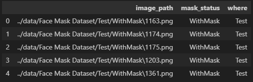

데이터 확인

print("With Mask:", dataset.value_counts("mask_status")[0])
print("Without Mask:", dataset.value_counts("mask_status")[1])

sns.countplot(x=dataset["mask_status"])
-----------------------------------------
With Mask: 5909
Without Mask: 5883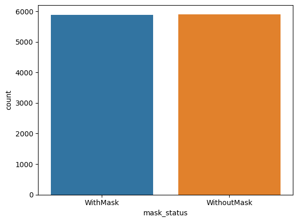

import cv2

plt.figure(figsize=(15,10))
for i in range(9):
    random = np.random.randint(1, len(dataset))
    plt.subplot(3, 3, i+1)
    plt.imshow(cv2.imread(dataset.loc[random, "image_path"]))
    plt.title(dataset.loc[random, "mask_status"], size=15)
    plt.xticks([]); plt.yticks([])
plt.show()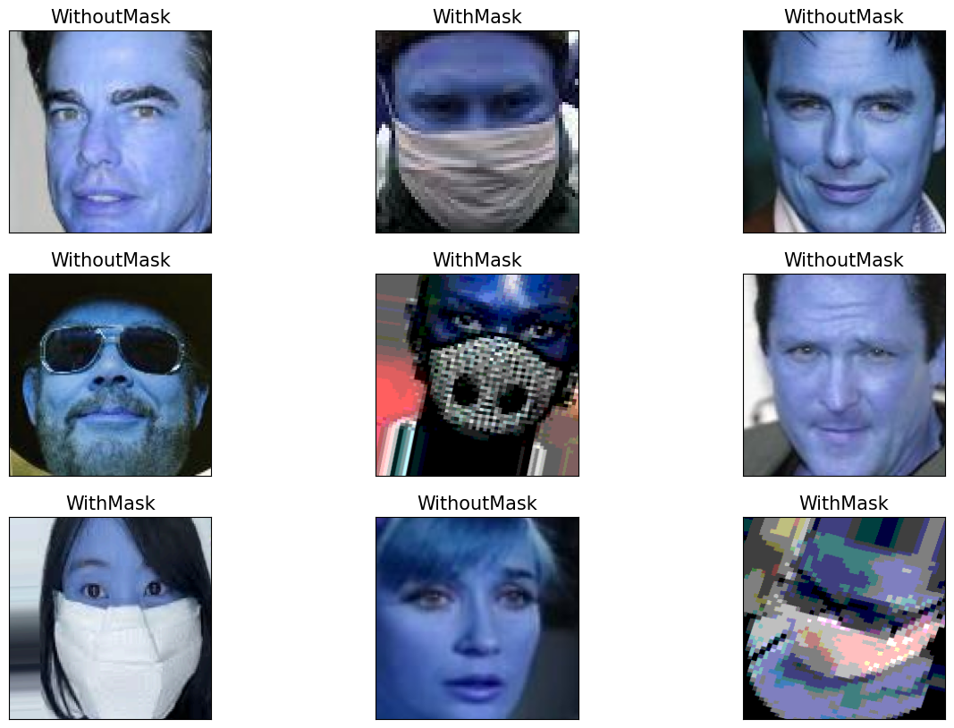

train_df = dataset[dataset["where"]=="Train"]
test_df = dataset[dataset["where"]=="Test"]
valid_df = dataset[dataset["where"]=="Validation"]

plt.figure(figsize=(15, 5))
plt.subplot(131)
sns.countplot(x=train_df["mask_status"])
plt.title("Train Dataset", size=10)

plt.subplot(132)
sns.countplot(x=test_df["mask_status"])
plt.title("test Dataset", size=10)

plt.subplot(133)
sns.countplot(x=valid_df["mask_status"])
plt.title("Validation Dataset", size=10)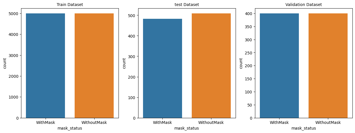

Data preprocessing

인덱스 초기화

train_df = train_df.reset_index(drop=True)
train_df.head()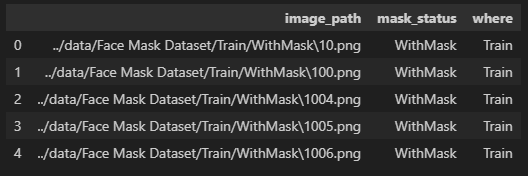

이미지 전처리

data = []
image_size = 150

for i in range(len(train_df)):
    # Converting the image into grayscale
    img_array = cv2.imread(train_df["image_path"][i], cv2.IMREAD_GRAYSCALE)
    
    # Resizing the array
    new_image_array = cv2.resize(img_array, (image_size, image_size))
    
    # Encoding the image with the label
    if train_df["mask_status"][i] == "WithMask":
        data.append([new_image_array, 1])
    else:
        data.append([new_image_array, 0])
        
np.random.shuffle(data)	# 순서를 학습하지 못하도록 shuffle

전처리 데이터 확인

fig, ax = plt.subplots(2, 3, figsize=(10,6))

for row in range(2):
    for col in range(3):
        image_index = row * 100 + col
        
        ax[row, col].axis("off")
        ax[row, col].imshow(data[image_index][0], cmap="gray")
        
        if data[image_index][1] == 0:
            ax[row, col].set_title("Without Mask")
        else:
            ax[row, col].set_title("With Mask")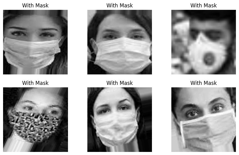

Modeling

모델 학습

X = []
y = []
for image in data:
    X.append(image[0])
    y.append(image[1])

X = np.array(X)
y = np.array(y)

X_train, X_val, y_train, y_val = train_test_split(X, y, test_size=0.2, random_state=13)
model = models.Sequential([
    layers.Conv2D(32, kernel_size=(5,5), strides=(1,1), padding="same", activation="relu", input_shape=(150,150,1)),
    layers.MaxPooling2D(pool_size=(2,2), strides=(2,2)),
    layers.Conv2D(64, kernel_size=(2,2), padding="same", activation="relu"),
    layers.MaxPooling2D(pool_size=(2,2)),
    layers.Dropout(0.25),
    layers.Flatten(),
    layers.Dense(1000, activation="relu"),
    layers.Dense(1, activation="sigmoid")              
])

model.compile(optimizer="adam", loss=tf.keras.losses.BinaryCrossentropy(), metrics=["accuracy"])

X_train = X_train.reshape(X_train.shape[0], X_train.shape[1], X_train.shape[2], 1)
X_val = X_val.reshape(X_val.shape[0], X_val.shape[1], X_val.shape[2], 1)
history = model.fit(X_train, y_train, epochs=4, batch_size=32)
---------------------------------------------------------------------------------------------------
Epoch 1/4
250/250 [==============================] - 317s 1s/step - loss: 25.5447 - accuracy: 0.8960
Epoch 2/4
250/250 [==============================] - 393s 2s/step - loss: 0.0632 - accuracy: 0.9758
Epoch 3/4
250/250 [==============================] - 379s 2s/step - loss: 0.0300 - accuracy: 0.9894
Epoch 4/4
250/250 [==============================] - 391s 2s/step - loss: 0.0185 - accuracy: 0.9933

Colab GPU 사용시 학습속도

모델 평가

모델 성능 확인

model.evaluate(X_val, y_val)
-----------------------------------------------------------------------------------------
63/63 [==============================] - 16s 253ms/step - loss: 0.1214 - accuracy: 0.9660
[0.12140300869941711, 0.9660000205039978]

prediction = (model.predict(X_val) > 0.5).astype("int32")

print(classification_report(y_val, prediction))
print(confusion_matrix(y_val, prediction))
----------------------------------------------------------------------------------------
63/63 [==============================] - 14s 222ms/step
              precision    recall  f1-score   support

           0       0.96      0.97      0.97      1032
           1       0.97      0.96      0.96       968

    accuracy                           0.97      2000
   macro avg       0.97      0.97      0.97      2000
weighted avg       0.97      0.97      0.97      2000

[[1001   31]
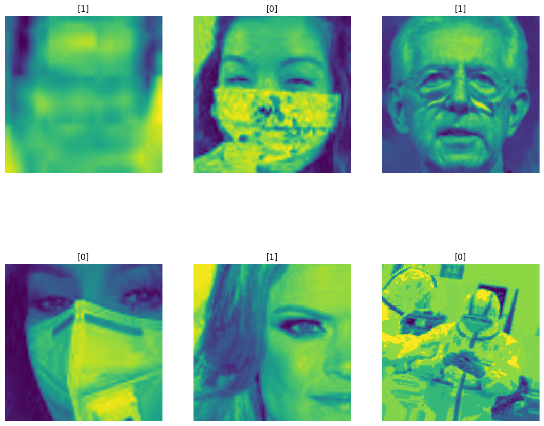
 [  37  931]]

틀린데이터 확인

wrong_result = []

for n in range(y_val.shape[0]):
    if prediction[n] != y_val[n]:
        wrong_result.append(n)

len(wrong_result)
-------------------------------------------------
68

import random

samples = random.choices(population=wrong_result, k=6)

plt.figure(figsize=(14, 12))

for idx, n in enumerate(samples):
    plt.subplot(2, 3, idx+1)
    plt.imshow(X_val[n].reshape(150, 150),interpolation="nearest")
    plt.title(prediction[n])
    plt.axis("off")