자료형
데이터의 성질
Python에서는 type()로 특정 데이터의 자료형 확인
print(type(10))
<class 'int'>

print(type(2.718))
<class 'float'>

print(type("hello"))
<class 'str'>
변수
알파벳을 사용하여 변수 정의
변수를 사용하여 계산하거나 변수에 다른 값을 대입
Python은 동적 언어로 변수의 자료형을 상황에 맞게 자동으로 결정
10이라는 정수로 초기화 할 때, x의 형태가 int임을 Python이 스스로 판단
정수와 실수를 곱한 결과는 실수(자동 형변환)
x=10
print(x)
10

x = 100
print(x)
100

y = 3.14
x * y
print(type(x * y))
<class 'float'>
리스트
[]안의 수를 인덱스, 인덱스는 0부터 시작
Python 리스트에는 Slicing이라는 편리한 기법 준비
Slicing을 이용하여 범위를 지정해 원하는 부분 리스트 획득
a = [1, 2, 3, 4, 5]
print(a)
[1, 2, 3, 4, 5]

print(len(a))
5

print(a[0])
1

print(a[4])
5

a[4] = 99
print(a)
[1, 2, 3, 4, 99]

print(a[0:2]) # 인덱스 0부터 2까지(2는 포함하지 않음)
[1, 2]

print(a[1:]) # 인덱스 1부터 끝까지
[2, 3, 4, 99]

print(a[:3]) # 인덱스 처음부터 3까지(3은 포함하지 않음)
[1, 2, 3]

print(a[:-1]) # 인덱스 처음부터 마지막 원소의 1개 앞까지
[1, 2, 3, 4]

print(a[:-2]) # 인덱스 처음부터 마지막 원소의 2개 앞까지
[1, 2, 3]
딕셔너리
리스트는 인덱스 번호로 값을 저장
딕셔너리는 Key와 Value를 한 쌍으로 저장
me = {'height':180}
print(me)
{'height': 180}

print(me['height'])
180

me['weight'] = 70
print(me)
{'height': 180, 'weight': 70}
bool
이 자료형은 True와 False라는 두 값 중 하나를 취함
bool에는 and, or, not 연산자 사용 가능
hungry = True
sleepy = False
print(type(hungry))
<class 'bool'>

print(not hungry)
False

print(hungry and sleepy)
False

print(hungry or sleepy)
True
if문
조건에 따라서 달리 처리하려면 if/else문 사용
Python에서는 공백 문자가 중요한 의미
if 문에서도 다음 줄은 앞쪽에 4개의 공백 문자로 들여쓰기
Python에서는 Tab 보다는 공백 문자 쪽을 권장
hungry = True
if hungry:
  print("I'm hungry")

I'm hungry

hungry = False
if hungry:
  print("I'm hungry")
else:
  print("Im'not hungry")
  print("I'm sleepy")

Im'not hungry
I'm sleepy
for문
반복 처리
for i in [1, 2, 3]:
  print(i)

1
2
3
함수
특정 기능을 수행하는 일련의 명령들을 묶어 하나의 함수로 정의
함수는 인자를 취할 수 있고, + 연산자를 사용하여 문자열을 이어 붙일 수 있음
def hello():
  print("Hello World!")
hello()

Hello World!

def hello(object):
  print("Hello " + object + "!")
hello("cat")

Hello cat!
클래스
Python에서는 class라는 keyword를 사용하여 클래스틑 정의
__init__ method는 클래스 초기화 방법을 정의하며, 생성자라고 함
클래스의 Instance가 만들어질 때 한 번만 호출
Python에서는 methom의 첫 번째 인수로 자신의 Instance를 나타내는 self를 명시적으로 쓰는 것이 특징
Instance 변수는 Instance 별로 저장
class Man:
  def __init__(self, name):
    self.name = name # self.name을 초기화, Instance 변수
    print("Initialized!")

  def hello(self):
    print("Hello " + self.name + "!")

  def goodbye(self):
    print("Good-bye " + self.name + "!")
m = Man("David")
Initialized!
m.hello()
Hello David!
m.goodbye()
Good-bye David!넘파이
딥러닝 구현 시 배열이나 행렬 계산이 많이 필요
넘파이의 배열 클래스인 numpy.array에는 편리한 method가 많이 준비
딥러닝 구현 시 이 method들을 이용
#넘파이 가져오기, numpy를 np라는 이름으로 import
import numpy as np
넘파이 배열 생성하기
#np.array() method로 넘파이 배열 생성
#인수로 Python의 리스트를 사용하여 넘파이가 제공하는 numpy.ndarray 배열을 반환
x = np.array([1.0, 2.0, 3.0])
print(x)
[1. 2. 3.]

print(type(x))
<class 'numpy.ndarray'>
넘파이 배열로 산술 연산 수행 예제
배열 x와 y의 원소 수가 같아야 함
원소별 곱셈 : element-wise product
x = np.array([1.0, 2.0, 3.0])
y = np.array([2.0, 4.0, 6.0])
print(x + y)
[3. 6. 9.]

print(x - y)
[-1. -2. -3.]

print(x * y)
[ 2.  8. 18.]

print(x / y)
[0.5 0.5 0.5]
넘파이 N차원 배열
넘파이는 1차원 배열 뿐 아니라 다차원 배열도 작성 가능
1차원 배열은 Vector
2차원 배열은 Matrix
Vector와 Matrix를 일반화한 것을 Tensor
A = np.array([[1, 2], [3, 4]])
print(A)
[[1 2]
 [3 4]]

print(A.shape) # 행렬의 형상
(2, 2)

print(A.dtype) # 행렬에 담긴 원소의 자료형
int64

B = np.array([[3, 0], [0, 6]])
print(A + B)
[[ 4  2]
 [ 3 10]]

print(A * B)
[[ 3  0]
 [ 0 24]]
브로드캐스트
넘파이 배열은 element-wise 계산 뿐만 아니라 넘파이 배열과 스칼라값(수치 하나)의 조합으로된 산술 연산도 수행 가능
스칼라값과의 계산이 넘파이 배열의 원소별로 한 번씩 수행
스칼라값이 넘파이 배열의 행렬에 맞게 확대된 후 연산
x = np.array([1.0, 2.0, 3.0])
print(x / 2.0)
[0.5 1.  1.5]

#1차원 배열은 B가 2차원 배열인 A와 똑같은 shape으로 변형된 후 element-wise 연산 수행
A = np.array([[1, 2], [3, 4]])
B = np.array([10, 20])
print(A * B)
[[10 40]
 [30 80]]
넘파이 원소 접근
X = np.array([[51, 55], [14, 19], [0, 4]])
print(X)
[[51 55]
 [14 19]
 [ 0  4]]

print(X[0])
[51 55]

print(X[0][1])
55

for row in X:
  print(row)
[51 55]
[14 19]
[0 4]

X = X.flatten() # X를 1차원 배열로 변환
print(X)
[51 55 14 19  0  4]

print(X[np.array([0, 2, 4])])
[51 14  0]
matplotlib
딥러닝 실험에서는 그래프 그리기와 데이터 시각화도 중요
matplotlib는 그래프를 그려주는 라이브러리
sin함수 예제
import numpy as np
import matplotlib.pyplot as plt

x = np.arange(0, 6, 0.1) # 0에서 6까지 X 축을 0.1 간격으로 생성
print(x)
[0.  0.1 0.2 0.3 0.4 0.5 0.6 0.7 0.8 0.9 1.  1.1 1.2 1.3 1.4 1.5 1.6 1.7
 1.8 1.9 2.  2.1 2.2 2.3 2.4 2.5 2.6 2.7 2.8 2.9 3.  3.1 3.2 3.3 3.4 3.5
 3.6 3.7 3.8 3.9 4.  4.1 4.2 4.3 4.4 4.5 4.6 4.7 4.8 4.9 5.  5.1 5.2 5.3
 5.4 5.5 5.6 5.7 5.8 5.9]

y = np.sin(x)

plt.plot(x, y)
plt.show()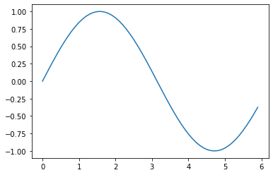
cos함수 예제
import numpy as np
import matplotlib.pyplot as plt

x = np.arange(0, 6, 0.1)
y1 = np.sin(x)
y2 = np.cos(x)

plt.plot(x, y1, label="sin")
plt.plot(x, y2, linestyle="--", label="cos") # cos 함수는 점섬으로 그리기
plt.xlabel("x")
plt.ylabel("y")
plt.title('sin & cos') # 제목
plt.legend() # 범례 표시
plt.show()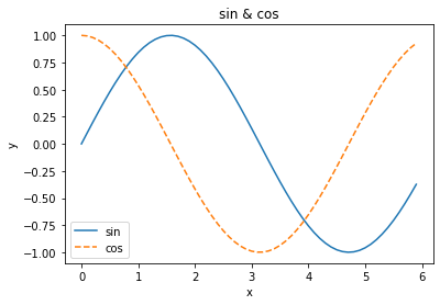
이미지 표시하기
pyplot에는 이미지를 표시해주는 method인 imshow() 사용
이미지를 읽어들일 때는 matplotlib.image 모듈의 imread() method 이용
import matplotlib.pyplot as plt
from matplotlib.image import imread

img = imread('/content/drive/MyDrive/lena.png')

plt.imshow(img)
plt.show()
참고
colab notebook을 사용할 때 런타임 인스턴스에 업로드 한 파일은 인스턴스가 다시 실행될 때 제거되므로 Google Drive를 마운트하여 마운트한 경로에 파일을 업로드한 후 경로 지정
from google.colab import drive
drive.mount('/content/drive')