Regularization
- 오버피팅을 해결하기 위한 방법입니다.
- L1, L2, Dropout, Batchnormalization등이 있습니다.
Normalization
- 데이터의 형태를 의미있게 바꿔주거나 전처리과정중 하나입니다.
- minmax scalar 같인 것이 있습니다.
from sklearn.datasets import load_iris
import pandas as pd
import matplotlib.pyplot as plt

iris = load_iris()
iris_df = pd.DataFrame(data=iris.data, columns=iris.feature_names)
target_df = pd.DataFrame(data=iris.target, columns=['species'])

# 0, 1, 2로 되어있는 target 데이터를
# 알아보기 쉽게 'setosa', 'versicolor', 'virginica'로 바꿉니다
def converter(species):
    if species == 0:
        return 'setosa'
    elif species == 1:
        return 'versicolor'
    else:
        return 'virginica'

target_df['species'] = target_df['species'].apply(converter)

iris_df = pd.concat([iris_df, target_df], axis=1)
iris_df.head()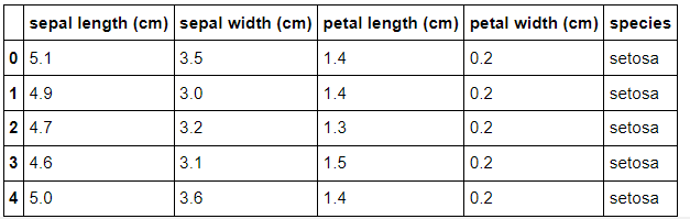
X= petal length, Y = sepal length
X = [iris_df['petal length (cm)'][a] for a in iris_df.index if iris_df['species'][a]=='virginica']
Y = [iris_df['sepal length (cm)'][a] for a in iris_df.index if iris_df['species'][a]=='virginica']

print(X)
print(Y)
X, Y를 그래프로 확인해보겠습니다.
plt.figure(figsize=(5,5))
plt.scatter(X,Y)
plt.title('petal-sepal scatter before normalization')
plt.xlabel('petal length (cm)')
plt.ylabel('sepal length (cm)')
plt.grid()
plt.show()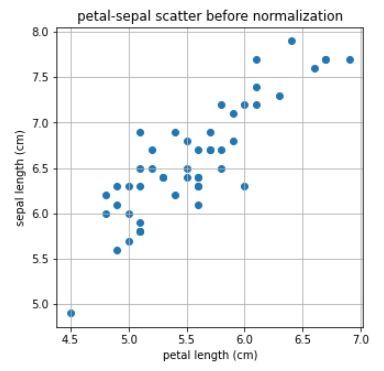
이제 0-1로 normlization을 해주는 minmax_scale를 이용해서 산점도를 다시 한번 그려보겠습니다.
from sklearn.preprocessing import minmax_scale

X_scale = minmax_scale(X)
Y_scale = minmax_scale(Y)

plt.figure(figsize=(5,5))
plt.scatter(X_scale,Y_scale)
plt.title('petal-sepal scatter after normalization')
plt.xlabel('petal length (cm)')
plt.ylabel('sepal length (cm)')
plt.grid()
plt.show()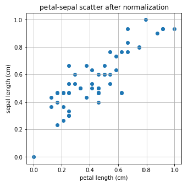
sklearn.linear_model에 포함된 LinearRegression 모델을 사용하여 X-Y 관계를 선형으로 모델링 해 보겠습니다.
from sklearn.linear_model import LinearRegression
import numpy as np

X = np.array(X)
Y = np.array(Y)

# Iris Dataset을 Linear Regression으로 학습합니다.
linear= LinearRegression()
linear.fit(X.reshape(-1,1), Y)

# Linear Regression의 기울기와 절편을 확인합니다.
a, b=linear.coef_, linear.intercept_
print("기울기 : %0.2f, 절편 : %0.2f" %(a,b))
기울기 : 1.00, 절편 : 1.06
plt.figure(figsize=(5,5))
plt.scatter(X,Y)
plt.plot(X,linear.predict(X.reshape(-1,1)),'-b')
plt.title('petal-sepal scatter with linear regression')
plt.xlabel('petal length (cm)')
plt.ylabel('sepal length (cm)')
plt.grid()
plt.show()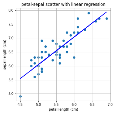
L1 regularization를 보겠습니다
#L1 regularization은 Lasso로 import 합니다.
from sklearn.linear_model import Lasso

L1 = Lasso()
L1.fit(X.reshape(-1,1), Y)
a, b=L1.coef_, L1.intercept_
print("기울기 : %0.2f, 절편 : %0.2f" %(a,b))

plt.figure(figsize=(5,5))
plt.scatter(X,Y)
plt.plot(X,L1.predict(X.reshape(-1,1)),'-b')
plt.title('petal-sepal scatter with L1 regularization(Lasso)')
plt.xlabel('petal length (cm)')
plt.ylabel('sepal length (cm)')
plt.grid()
plt.show()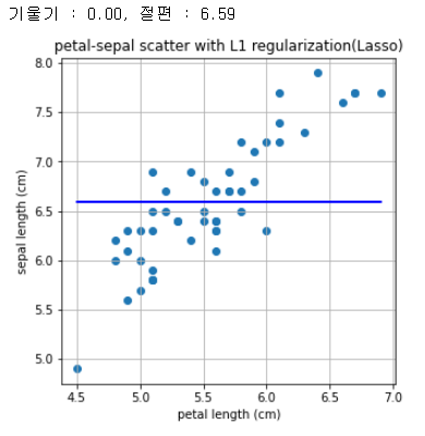
L2 regularization
#L2 regularization은 Ridge로 import 합니다.
from sklearn.linear_model import Ridge

L2 = Ridge()
L2.fit(X.reshape(-1,1), Y)
a, b = L2.coef_, L2.intercept_
print("기울기 : %0.2f, 절편 : %0.2f" %(a,b))

plt.figure(figsize=(5,5))
plt.scatter(X,Y)
plt.plot(X,L2.predict(X.reshape(-1,1)),'-b')
plt.title('petal-sepal scatter with L2 regularization(Ridge)')
plt.xlabel('petal length (cm)')
plt.ylabel('sepal length (cm)')
plt.grid()
plt.show()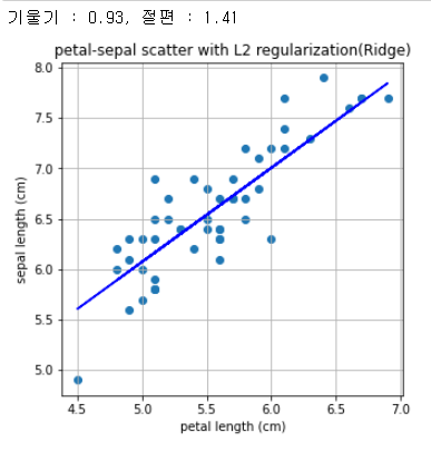
Dropout
확률적으로 랜덤하게 몇 가지의 뉴럴만 선택하여 정보를 전달하는 과정입니다.
import tensorflow as tf
from tensorflow import keras
import numpy as np
import matplotlib.pyplot as plt
from sklearn.model_selection import train_test_split

fashion_mnist = keras.datasets.fashion_mnist
(train_images, train_labels), (test_images, test_labels) = fashion_mnist.load_data()
class_names = ['T-shirt/top', 'Trouser', 'Pullover', 'Dress', 'Coat',
'Sandal', 'Shirt', 'Sneaker', 'Bag', 'Ankle boot']
train_images = train_images / 255.0
test_images = test_images / 255.0
model = keras.Sequential([
    keras.layers.Flatten(input_shape=(28, 28)),
    keras.layers.Dense(128, activation='relu'),
    # 여기에 dropout layer를 추가해보았습니다. 나머지 layer는 아래의 실습과 같습니다.
    keras.layers.Dropout(0.9),
    keras.layers.Dense(10, activation='softmax')
])

model.compile(optimizer='adam',loss='sparse_categorical_crossentropy',
              metrics=['accuracy'])

history= model.fit(train_images, train_labels, epochs=5)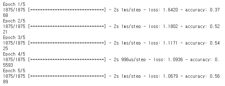
model = keras.Sequential([
    keras.layers.Flatten(input_shape=(28, 28)),
    # 이번에는 dropout layer가 없습니다.
    keras.layers.Dense(128, activation='relu'),
    keras.layers.Dense(10, activation='softmax')
])

model.compile(optimizer='adam',loss='sparse_categorical_crossentropy',
              metrics=['accuracy'])

history = model.fit(train_images, train_labels, epochs=5)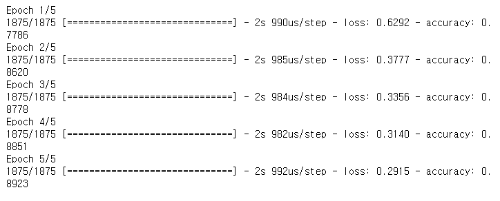
Batch Normalization
fully connected layer와 Batch Normalization layer를 보겠습니다.
import tensorflow as tf
from tensorflow import keras
import numpy as np
import matplotlib.pyplot as plt

fashion_mnist = keras.datasets.fashion_mnist
(train_images, train_labels), (test_images, test_labels) = fashion_mnist.load_data()
class_names = ['T-shirt/top', 'Trouser', 'Pullover', 'Dress', 'Coat',
'Sandal', 'Shirt', 'Sneaker', 'Bag', 'Ankle boot']
train_images = train_images / 255.0
test_images = test_images / 255.0from sklearn.model_selection import train_test_split
X_train, X_valid, y_train, y_valid = train_test_split(train_images, train_labels, test_size=0.3, random_state=101)
model = keras.Sequential([
keras.layers.Flatten(input_shape=(28, 28)),
keras.layers.Dense(128, activation='relu'),
#여기에 batchnormalization layer를 추가해보았습니다. 나머지 layer는 위의 실습과 같습니다.
keras.layers.BatchNormalization(),
keras.layers.Dense(10, activation='softmax')
])
model.compile(optimizer='adam',loss='sparse_categorical_crossentropy',
metrics=['accuracy'])
history= model.fit(X_train, y_train, epochs=20, batch_size=2048, validation_data=(X_valid, y_valid))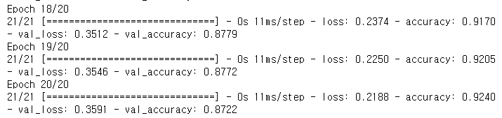
# loss 값을 plot 해보겠습니다.
y_vloss = history.history['val_loss']
y_loss = history.history['loss']
x_len = np.arange(len(y_loss))

plt.plot(x_len, y_vloss, marker='.', c='red', label="Validation-set Loss")
plt.plot(x_len, y_loss, marker='.', c='blue', label="Train-set Loss")
plt.legend(loc='upper right')
plt.grid()
plt.ylim(0,1)
plt.title('Loss graph with batch normalization')
plt.xlabel('epoch')
plt.ylabel('loss')
plt.show()
# accuracy 값을 plot 해보겠습니다.
y_vacc = history.history['val_accuracy']
y_acc = history.history['accuracy']
x_len = np.arange(len(y_acc))

plt.plot(x_len, y_vacc, marker='.', c='red', label="Validation-set accuracy")
plt.plot(x_len, y_acc, marker='.', c='blue', label="Train-set accuracy")
plt.legend(loc='lower right')
plt.grid()
plt.ylim(0.5,1)
plt.title('Accurcy graph with batch normalization')
plt.xlabel('epoch')
plt.ylabel('accuracy')
plt.show()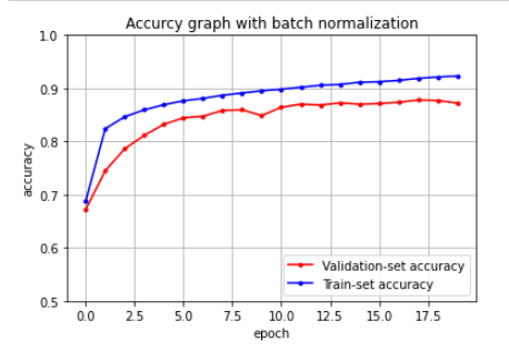

인공지능 파이팅!