module import
import yfinance as yf
import pandas as pd
import numpy as np

import matplotlib.pyplot as plt
import seaborn as sns
sns.set_style('whitegrid')
plt.style.use("fivethirtyeight")

import pandas_datareader.data as datareader
import yfinance as yf

from datetime import datetime
investor_df = pd.read_parquet('investor.parquet')
investor_df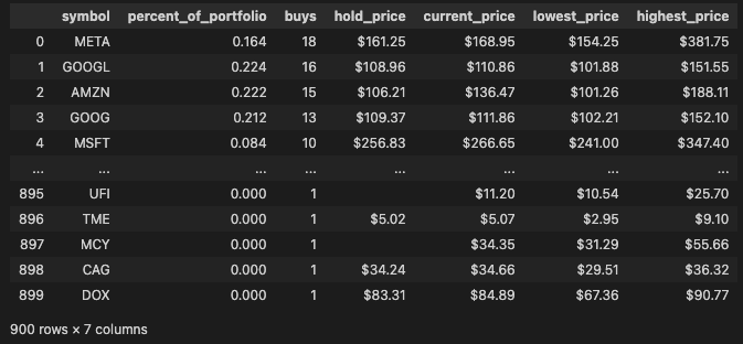
살펴볼 데이터 추려내기
- 지난 분기에 가장 많은 구매자 순서로 9개의 종목만 추려보도록 한다
1. ROE(Return of Equity)
- 기업이 자본을 이용하여 얼마만큼의 이익을 냈는지를 나타내는 지표
- 추후에 사용할 수 있는 지표로, 미리 데이터프레임에 넣어둔다
tech_list = ['META','GOOGL','AMZN', 'GOOG', 'MSFT','DIS','BKNG', 'PYPL','NFLX']
roe_list = []
for i in tech_list:
    try:
        val = yf.Ticker(i).info['returnOnEquity']
        roe_list.append(val)
    except:
        roe_list.append(np.NaN)
        pass
2. EY(Earnings Yield)
- 기업에 지불해야하는 가격 대비 해당기업이 벌어 줄 수 있는 이윤의 비율
- EY(이익수익률) = 시가 총액 / 기업 가치
ey_list = []
for i in tech_list:
    try:
        val = yf.Ticker(i).info['marketCap'] / yf.Ticker(i).info['enterpriseValue']
        ey_list.append(val)
    except:
        ey_list.append(np.NaN)
        pass
sample_df = investor_df.head(9)
sample_df['ROE'] = roe_list
sample_df['EY'] = ey_list위의 작업들을 통해 완성된 데이터 프레임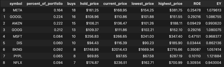
- 데이터를 살펴볼 날짜는
22년 6월 30일까지의 1년이다
start = date.fromisoformat('2021-07-01')
end = date.fromisoformat('2022-06-30')
for stock in tech_list:
globals()[stock] = yf.download(stock, start, end)- 살펴볼 종목들 확인 및 각 종목별 데이터프레임 만들기
company_list = [META, GOOGL, AMZN, GOOG, MSFT, DIS, BKNG, PYPL, NFLX]
company_name = ['META', 'GOOGLE-A','AMAZON', 'GOOGLE', 'MICROSOFT','DISNEY','BOOKING HOLDINGS','PAYPAL','NETFLIX']
for company, com_name in zip(company_list, company_name):
    company["company_name"] = com_name

df = pd.concat(company_list, axis=0)
EDA
1. Adj Close
plt.figure(figsize = (35, 15))
plt.subplots_adjust(top = 1.25, bottom = 1.2)

for i, company in enumerate(company_list, 1):
    plt.subplot(3, 3, i)
    company['Adj Close'].plot()
    plt.ylabel('Adj Close')
    plt.xlabel(None)
    plt.title(f"Closing Price of {tech_list[i - 1]}")
plt.tight_layout()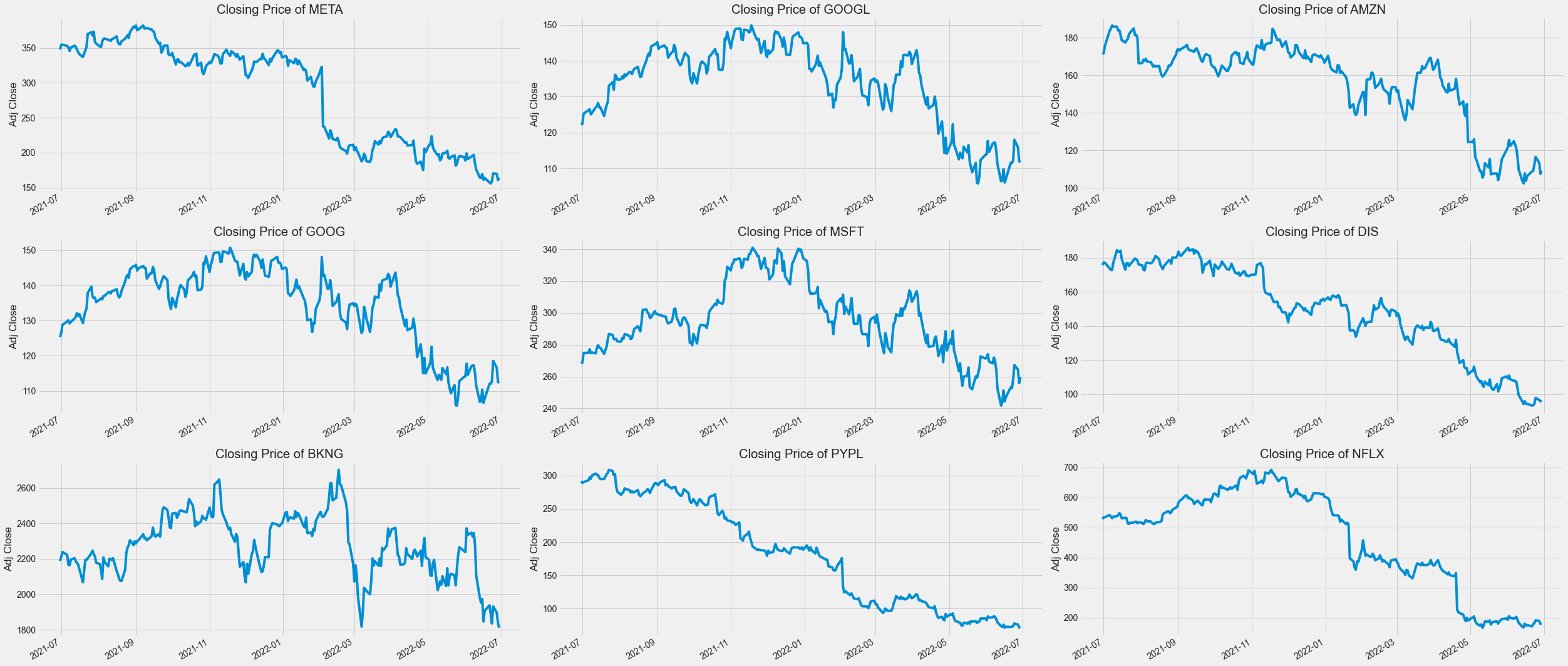
2. Volume
plt.figure(figsize=(35, 15))
plt.subplots_adjust(top=1.25, bottom=1.2)

for i, company in enumerate(company_list, 1):
    plt.subplot(3, 3, i)
    company['Volume'].plot()
    plt.ylabel('Volume')
    plt.xlabel(None)
    plt.title(f"Sales Volume for {tech_list[i - 1]}")

plt.tight_layout()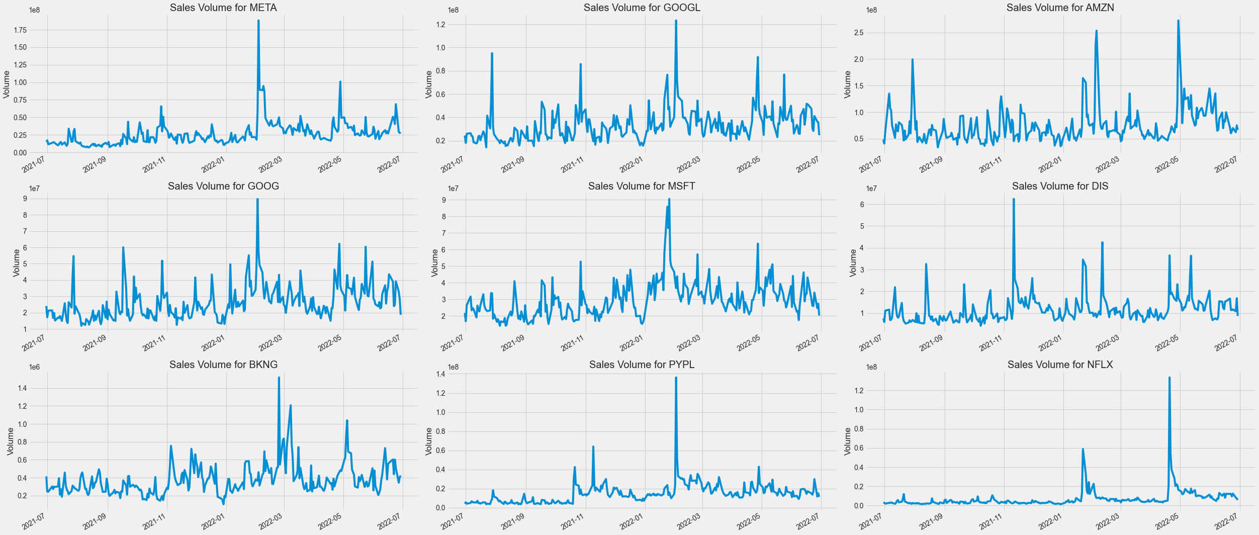
3. Moving average
- 주식시장이나 파생상품 시장에서 기술적 분석을 할 때 쓰이는 기본 도구 중 하나이다. 과거의 평균적 수치에서 현상을 파악하여 현재의 매매와 미래의 예측에 접목할 수 있도록 돕는다
ma_day = [10, 20, 50]

for ma in ma_day:
    for company in company_list:
        column_name = f"MA for {ma} days"
company[column_name] = company['Adj Close'].rolling(ma).mean()fig, ax = plt.subplots(nrows = 3, ncols = 3)
fig.set_figheight(12)
fig.set_figwidth(25)
META[['Adj Close','MA for 10 days', 'MA for 20 days', 'MA for 50 days']].plot(ax = ax[0,0])
ax[0,0].set_title('META')
GOOGL[['Adj Close','MA for 10 days', 'MA for 20 days', 'MA for 50 days']].plot(ax = ax[0,1])
ax[0,1].set_title('GOOGL')
AMZN[['Adj Close','MA for 10 days', 'MA for 20 days', 'MA for 50 days']].plot(ax = ax[0,2])
ax[0,2].set_title('AMZN')
GOOG[['Adj Close','MA for 10 days', 'MA for 20 days', 'MA for 50 days']].plot(ax = ax[1,0])
ax[1,0].set_title('GOOG')
MSFT[['Adj Close','MA for 10 days', 'MA for 20 days', 'MA for 50 days']].plot(ax = ax[1,1])
ax[1,1].set_title('MSFT')
DIS[['Adj Close','MA for 10 days', 'MA for 20 days', 'MA for 50 days']].plot(ax = ax[1,2])
ax[1,2].set_title('DIS')
BKNG[['Adj Close','MA for 10 days', 'MA for 20 days', 'MA for 50 days']].plot(ax = ax[2,0])
ax[2,0].set_title('BKNG')
PYPL[['Adj Close','MA for 10 days', 'MA for 20 days', 'MA for 50 days']].plot(ax = ax[2,1])
ax[2,1].set_title('PYPL')
NFLX[['Adj Close','MA for 10 days', 'MA for 20 days', 'MA for 50 days']].plot(ax = ax[2,2])
ax[2,2].set_title('NFLX')
fig.tight_layout()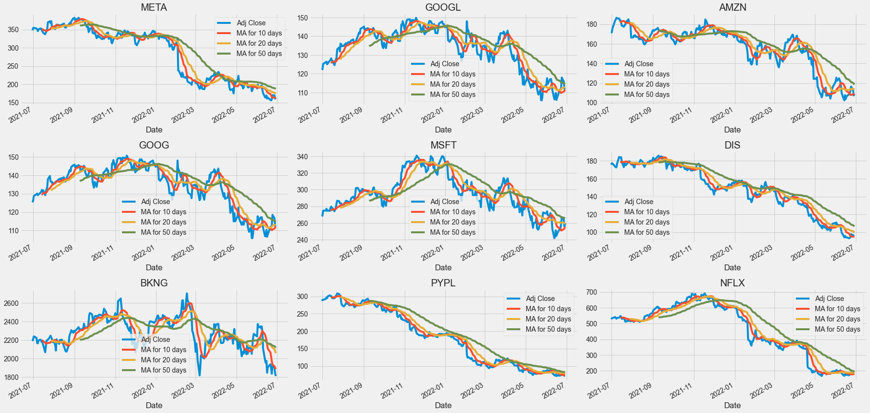
for company in company_list:
    company['Daily Return'] = company['Adj Close'].pct_change()

fig, ax = plt.subplots(nrows = 3, ncols = 3)
fig.set_figheight(12)
fig.set_figwidth(25)

META['Daily Return'].plot(ax = ax[0,0], legend=True, linestyle='--', marker='o')
ax[0,0].set_title('META')
GOOGL['Daily Return'].plot(ax = ax[0,1], legend=True, linestyle='--', marker='o')
ax[0,1].set_title('GOOGL')
AMZN['Daily Return'].plot(ax = ax[0,2], legend=True, linestyle='--', marker='o')
ax[0,2].set_title('AMZN')
GOOG['Daily Return'].plot(ax = ax[1,0], legend=True, linestyle='--', marker='o')
ax[1,0].set_title('GOOG')
MSFT['Daily Return'].plot(ax = ax[1,1], legend=True, linestyle='--', marker='o')
ax[1,1].set_title('MSFT')
DIS['Daily Return'].plot(ax = ax[1,2], legend=True, linestyle='--', marker='o')
ax[1,2].set_title('DIS')
BKNG['Daily Return'].plot(ax = ax[2,0], legend=True, linestyle='--', marker='o')
ax[2,0].set_title('BKNG')
PYPL['Daily Return'].plot(ax = ax[2,1], legend=True, linestyle='--', marker='o')
ax[2,1].set_title('PYPL')
NFLX['Daily Return'].plot(ax = ax[2,2], legend=True, linestyle='--', marker='o')
ax[2,2].set_title('NFLX')

fig.tight_layout()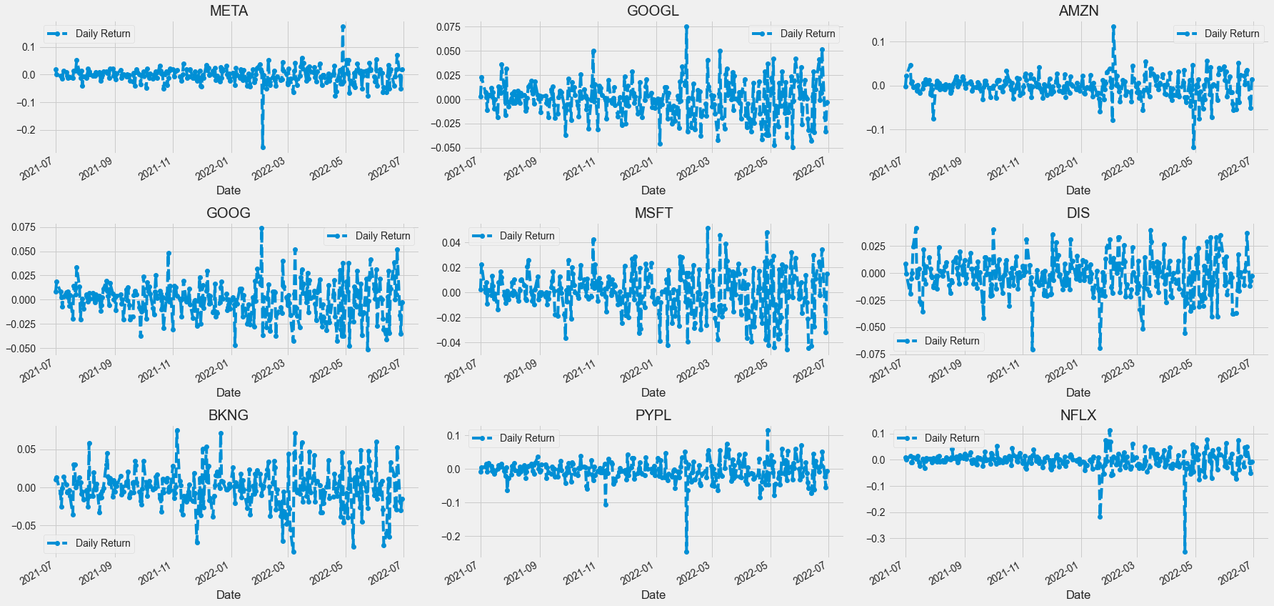
4. Daily Return
- 전날 대비 수익률
plt.figure(figsize = (20, 10))

for i, company in enumerate(company_list, 1):
    plt.subplot(3, 3, i)
    company['Daily Return'].hist(bins=50)
    plt.ylabel('Daily Return')
    plt.title(f'{company_name[i - 1]}')

plt.tight_layout()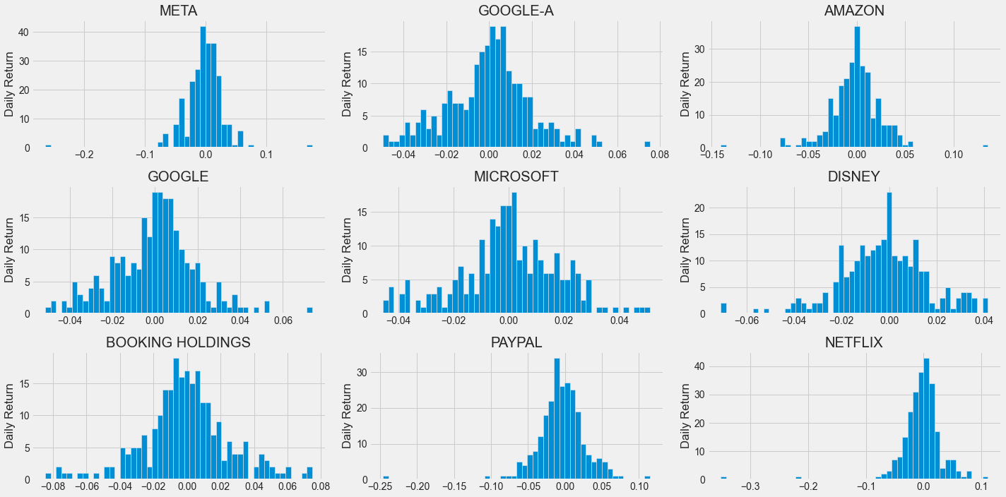
5. 각 종목별 상관계수 확인
closing_df = datareader.DataReader(tech_list, 'yahoo', start, end)['Adj Close']
closing_df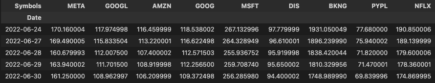
return_df = closing_df.pct_change()
return_df.tail()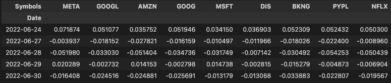
sns.pairplot(return_df, kind='reg')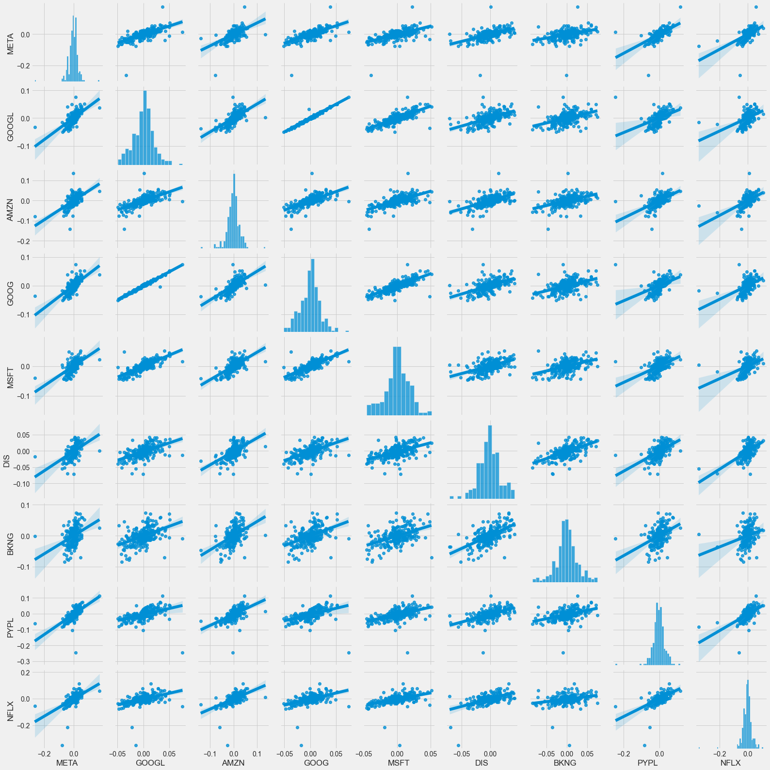
sns.heatmap(return_df.corr(), annot=True, cmap='summer')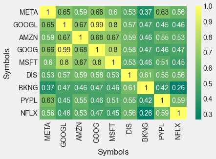
sns.heatmap(closing_df.corr(), annot=True, cmap='summer')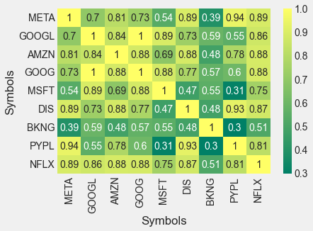
Modeling 준비
- 첫번째로 확인할 종목은, 가장 많은 구매자가 있었던 META로 한다
df = datareader.DataReader('META', data_source='yahoo', start='2021-06-30',end='2022-06-30')plt.figure(figsize = (20, 8))
plt.title('Close Price History')
plt.plot(df['Close'])
plt.xlabel('Date', fontsize = 18)
plt.ylabel('Close Price USD ($)', fontsize = 18)
plt.show()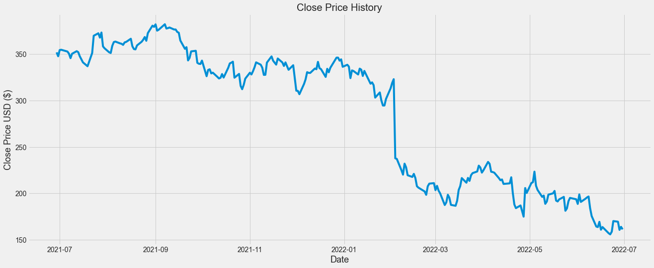
- 마감 가격으로 데이터 학습
from sklearn.preprocessing import MinMaxScaler

data = df.filter(['Close'])

dataset = data.values

training_data_len = int(np.ceil(len(dataset) * .95))

scaler = MinMaxScaler(feature_range=(0, 1))
scaled_data = scaler.fit_transform(dataset)
train_data = scaled_data[0: int(training_data_len), :]
x_train = []
y_train = []
for i in range(30, len(train_data)):
x_train.append(train_data[i - 30 : i, 0])
y_train.append(train_data[i, 0])
x_train, y_train = np.array(x_train), np.array(y_train)
x_train = np.reshape(x_train, (x_train.shape[0], x_train.shape[1], 1))LSTM 모델에 학습
from keras.models import Sequential
from keras.layers import Dense, LSTM

# 모델 빌드
model = Sequential()
model.add(LSTM(128, return_sequences=True, input_shape= (x_train.shape[1], 1)))
model.add(LSTM(64, return_sequences=False))
model.add(Dense(25))
model.add(Dense(1))

# 모델 컴파일
model.compile(optimizer='adam', loss='mean_squared_error')

# 모델 학습
model.fit(x_train, y_train, batch_size=1, epochs=1)
test_data = scaled_data[training_data_len - 30: , :]
x_test = []
y_test = dataset[training_data_len:, :]
print(test_data)
for i in range(30, len(test_data)):
x_test.append(test_data[i - 30 : i, 0])
x_test = np.array(x_test)
x_test = np.reshape(x_test, (x_test.shape[0], x_test.shape[1], 1))
predictions = model.predict(x_test)
predictions = scaler.inverse_transform(predictions)
rmse = np.sqrt(np.mean(((predictions - y_test) ** 2)))결과 확인
train = data[:training_data_len]
valid = data[training_data_len:]
valid['Predictions'] = predictions

plt.figure(figsize=(16,6))
plt.title('Model')
plt.xlabel('Date', fontsize = 18)
plt.ylabel('Close Price USD ($)', fontsize = 18)
plt.plot(train['Close'])
plt.plot(valid[['Close','Predictions']])
plt.legend(['Train','Val','Predictions'], loc = 'upper right')
plt.show()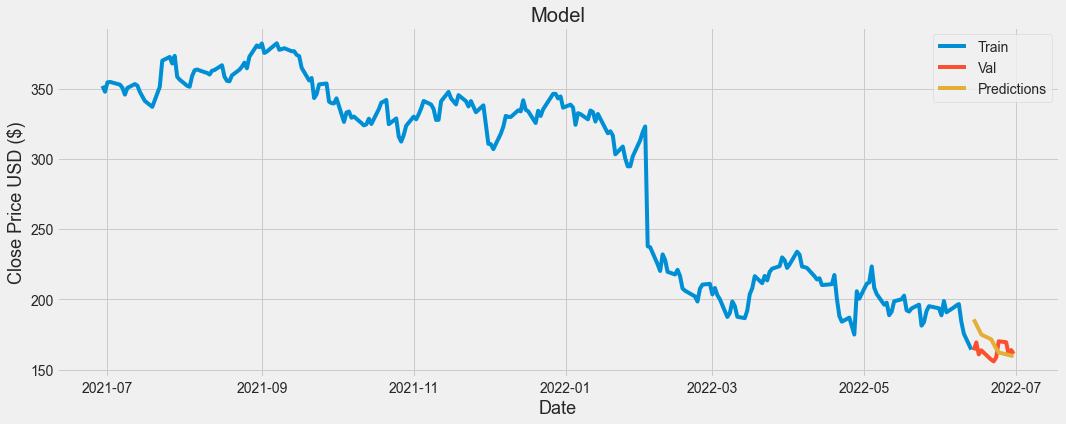
회고
우선, 시장 종가의 흐름을 가지고 다음날, 다음주, 다음달의 가격을 예측하는 것은 터무니 없는 소리라고 생각하는 계기가 되었다. 시계열 데이터로, '현재까지의 흐름으로 미루어 보아 다음엔 이럴것이다'라는 것을 예측하는 것은, 아무런 근거가 없다
- 우선, 시장 종가로 미래를 예측하는 것은, 어디에나 적용되는 행위가 아니다. 위의 종목별
Daily Return을 보면 알겠지만, 전날 대비 변화율이 그렇게 높지 않다. 결국 2%의 변화가 있다고 하더라도, 예측률이 98%인 모델이 되는 것이다. 하지만 이 2%가 모이면 그 변화량은 절대 무시하지 못한다 - 시장 종가 + 다른 종목과의 상관관계로 무언가를 알아내고자 하였지만, 자세히 들여다보면, 주식 시장이라는 큰 틀 안에서 각 종목은 어느정도 틀 안에서 논다. 경제가 박살나면 주가가 떨어지고, 시장이 활성화되면 모든 종목은 전체적으로 주가가 오르게 된다. 결국 중요한 것은, 다른 종목과의 상관관계가 아니라, 이 주식 시장의 활성화를 결정짓는 그 무언가인 것이다
- 미래를 예측하지 못한다. 미래 가격을 예측하기 위해 깃허브, 캐글, 구글 등 많은 코드들을 뒤져봤지만, 그 어디에도 종가를 이용하여 미래를 예측하는 것은 없었다. 자세히 들여다보면 사실상 과거로 돌아가, 모델이 말해주는 흐름을 볼 뿐이다.
종가를 이용한 시장 가격 예측에 실패한 것이다. 위에서 언급했듯, 시장을 움직이는 큰 틀에 대한 데이터 + 조엘 그린블라트의 퀀트 투자 전략을 이용하면 유의미한 데이터를 발굴할 수 있을거라 생각한다

데이터 엔지니어로 전향중인 백엔드 개발자입니다