Propensity score 성향점수
-연구 대상이 특정 공변량에 의해 대조군이 아니고 실험군에 포함될 확률
Propensity Score matching을 적용한 이후에는 bias를 좀 완화할 수 있는 model을 형성할 수 있음
기본 가정
1) conditional independence assumption
한 연구대상이 실험군에 속하게 되는 것은 관찰된 특징들에 의해 결정되어야 한다. 만약 관찰되지 않은 요인이 존재하면, matching estimator가 bias(편향)
2) common support condition (overlap condition)
비교를 시행하는 두 군의 propensity score들은 반드시 어느정도 중복되는 분포를 가지고 있어야 한다.
연구대상이 처치군과 대조군과 만약 random으로 배정된다고 가정하면, propensity score는 0.5 지만, 실제 준실험 설계에서 무작위 배정은 불가능하므로 각 공변량에 대한 propensity score를 추정하여 이 점수(확률)을 이용한 adjustment(조정)을 시행한다.
Propensity score는 공변량과 특정 처치를 받아 처치군에 포함되는 것과의 연관성에 따라 결정된다. 다른 공변량의 효과가 없다고 가정한다면, 특정 공변량에 대해 같은 propensity score를 가지는 연구대상들이 처치군과 대조군에 같은 수로 포함된다면 이 두 집단을 대상으로 한 통계적 추론의 결과는 같은 propensity score를 가지는 공변량에 의한 효과보다는 특정 처치를 받아 처치군에 포함되었기 때문에 발생한 차이에서 기인한 것이라고 할 수 있다.
Propensity Score 측정 방법
1)CART 이용 (복잡해서 잘 사용 안함) 2) Logistic model
2)번 방법은 실험군에 포함되는 경우를 1, 대조군에 포함되는 경우를 0으로 하는 이항반응(binary response) 형태로 종속변수를 설정하고, 보정하려는 공변량을 독립변수로 지정하여 로지스틱 회귀분석을 시행
이 경우 로지스틱 회귀분석은 propensity score model을 추정하며, 이 모형에 의해 각 대상들의 추정된 확률(각 대상이 주어진 공변량에 의해 처치군에 포함될 확률)이 propensity score에 해당된다. 이후 대조군과 처치군에 포함된 모든 연구대상에 대하여 propensity score가 같은 혹은 유사한 대상끼리 짝을 맞추어 자료를 선정하고 짝을 이루지 못한 것들은 분석에서 제외
R code 구현 예제
Treats <- subset(Data, Ad_Campaign_Response == 1)
##The treatment population
pscores.model <- glm(Ad_Campaign_Response ~ Age + Income,family = binomial("logit"),data = Data)
summary(pscores.model)
Propensity_scores <- pscores.model
Data $ PScores <- pscores.model $ fitted.values
hist(Data $ PScores[Ad_Campaign_Response==1],main = "PScores of Response = 1") ##HISTOGRAM DISTRIBUTION
hist(Data $ PScores[Ad_Campaign_Response==0], ,main = "PScores of Response = 0") #HISTOGRAM DISTRIBUTION
##Creating a Tableone pre-matching table
xvars <- c("Age", "Income")
library(tableone)
table1 <- CreateTableOne(vars = xvars,strata = "Ad_Campaign_Response",data = Data, test = FALSE)
print(table1, smd = TRUE)
##see the Standardized Mean Differences##596 subjects and in the treatment group there are 404 subjects in the control group
##SMD (Standardized Mean Difference)가 0.1 넘어가면 propensity matching이 필요함:)
전체적 Propensity Score Matching의 R 분석 flow
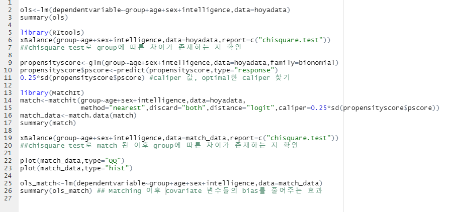
제 github에 code 업로드를 하였습니다:)
https://github.com/hoyajhl/R_stat/blob/main/propensityscore.R
추후에 정리해볼 내용들 (Propensity score advanced)
http://web.hku.hk/~bcowling/examples/propensity.htm
References
https://www.anesth-pain-med.org/journal/view.php?id=10.17085/apm.2016.11.2.130
https://www.kdnuggets.com/2018/01/propensity-score-matching-r.html
https://www.youtube.com/watch?v=jvyAW19oink