[Paper Review] Self-Attentive Sequential Recommendation
Kang, Wang-Cheng & McAuley, Julian. (2018). Self-Attentive Sequential Recommendation. 197-206. 10.1109/ICDM.2018.00035.
I. Introduction
Sequential recommender system의 목표는 유저 데이터로 학습된 모델을 유저의 최근 action에 기반한 context와 결합하는 것이다. 다만 유저의 action을 얼마나 오래 전부터 살펴볼 것인지에 따라 input 데이터 차원이 기하급수적으로 커지기 때문에 이러한 sequential dynamics로 유용한 패턴을 잡아내기는 어려운 일이다.
따라서 고차원의 데이터 속에서 간결하게 context를 뽑아내기 위한 많은 연구들이 이루어졌다. 대표적으로 Markov Chains(MCs)가 있는데, 유저의 다음 action은 직전 action에만 영향을 받는다는 가정을 바탕으로 추천시스템이 단기간의 item transition을 잘 학습하도록 했다. 이와 다르게 Recurrent Neural Networks(RNNs)는 hidden state를 통해 유저의 과거 모든 action을 바탕으로 유저의 다음 action을 예측하고자 했다. MC 기반 추천시스템은 높은 sparsity 상황에서도 잘 작동하지만 복잡한 상황에서의 action을 잘 학습하지 못한다는 단점이 있다. 반대로 RNN은 많은 양의 데이터를 필요로 하지만 간단한 모델보다 성능이 뛰어나다.
저자는 최근 번역 task에서 좋은 성능을 내고 있는 Transformer라는 sequential model에 영감을 받아 새로운 모델을 제안한다. Transformer는 self-attention이라고 불리는 attention 메커니즘을 이용해 문장에서 단어 사이의 의미적, 구조적 패턴을 효과적으로 찾아낸다. 이 self-attention 메커니즘을 sequential recommendation problems에 적용하여 RNN과 같이 유저의 과거 모든 action으로부터 context를 파악하고 MC처럼 적은 수의 action만으로 예측을 해내는 모델을 만들고자 했다. 그리고 모델을 Self-Attentive Sequential Recommendation(SASRec)이라고 이름 붙였다.
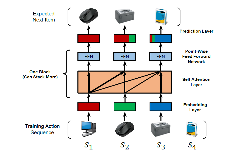
SASRec은 아래 그림처럼 각 time step마다 이전의 아이템에 대한 가중치를 조정한다.
attention 메커니즘의 영향으로, SASRec은 dense한 dataset에서는 긴 시간 범위의 의존성을 고려하고, sparse dataset에서는 최근 활동에 좀 더 집중하는 경향이 있다. 즉 density가 변하는 data 환경에 잘 적응할 수 있다는 것을 의미한다. 또한 parallel acceleration에 적합하기 때문에 CNN/RNN 계열의 모델보다 훨씬 빠른 학습 속도를 자랑한다.
II. Related Work
1. General Recommendation
일반적인 추천시스템은 과거 feedback에 기반하여 유저와 아이템 간의 양립성을 모델링한다. 이때 feedback은 평점과 같은 explicit한 것일 수도 있고, 클릭, 구매, 댓글처럼 implicit할 수도 있다. 그 중 implicit feedback을 모델링하기는 특히 더 어려운데, 관찰되지 않은 데이터를 해석하기가 모호하기 때문이다.
General Recommendation model로는 대표적으로 Matrix Factorization(MF)가 있다. MF는 유저와 아이템 embedding 간의 inner product로 유저와 아이템 간 interaction을 나타낸다. 또 Item Similarity Models(ISM)는 item-to-item similarity matrix를 학습해서 유저가 이전에 구매한 아이템과 비슷한 다른 아이템을 추천해준다.
최근에는 다양한 딥러닝 기술이 추천시스템이 적용되었다. context-aware recommendation에서 아이템 feature를 뽑아내기 위한 용도로 neural network를 사용하기도 하고, NeuMF나 AutoRec처럼 전통적인 MF를 대체하기 위해 neural network를 사용한 선행 연구도 존재한다.
2. Temporal Recommendation
Temporal Recommendation은 유저의 action 시간대를 명시적으로 모델링함으로써 다양한 task에서 좋은 성능을 보여주었다. TimeSVD++과 같은 temporal recommendation 모델들은 시간에 따른 단기 혹은 장기 추이가 있는 dataset을 이해하기 위해 필수적이다. Sequential recommendation은 시간에 관계없이 단순히 action의 순서만을 고려한다는 점에서 temporal recommendation과 차이가 있다.
3. Sequential Recommendation
Sequential Recommendation 모델은 구매로 이어진 아이템 사이의 순차적 패턴을 기반으로 item-item transition matrices를 모델링한다. first-order MC은 유저의 다음 action에 영향을 미치는 주요한 요소는 직전 아이템이라는 점에 착안하여, 특히 sparse한 dataset에서 좋은 성능을 보여주었다. high-order MC는 이전의 더 많은 아이템을 고려하는데, CNN 기반의 Convolutional Sequence Embedding에 적용되어 이전에 구매한 L개의 아이템에 대한 embedding matrix를 통해 convolutional operation을 수행하고 transition을 뽑아낸다.
MC 기반 모델 외에도, RNN을 이용해 유저 sequence를 모델링하는 선행 연구도 존재한다. 예를 들어 GRU4Rec은 session-based recommendation으로 클릭 sequence를 모델링한다. 각 time step에서 RNN은 직전 step의 state와 현재 action을 input으로 받는다.
4. Attention Mechanisms
Attention 메커니즘은 이미지 인식이나 번역과 같은 task에서 좋은 성능을 보여주었다. 근본적인 아이디어는 각 sequential output이 모델이 집중해야 할 몇몇 input에 영향을 받는다는 것이다. attention 메커니즘을 추천시스템에 적용시킨 선행 연구가 있긴 하지만 기존 모델에 추가적인 component를 추가한 것이 전부이다.
최근 Transformer라고 불리는 순수한 attention 기반의 sequence-to-sequence method가 번역 task에서 RNN/CNN 기반 모델을 압도했다. Transformer는 self-attention 모듈을 이용해 문장의 복잡한 구조를 이해하고 다음 단어를 생성하기 위해 연관 단어를 찾는다. 이러한 transformer에 영감을 받아 저자는 self-attention으로 새로운 sequential recommendation model을 제안한다.
III. Methodology
sequential recommendation에서는 유저의 action sequence 가 주어진 상태에서 다음 아이템을 예측한다. 즉 time step 의 모델은 이전 개 아이템에 의존하여 다음 아이템을 예측한다. 모델의 input을 , output을 으로 생각하면 된다.
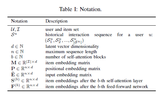
이외의 notation은 아래 표와 같다.
1. Embedding Layer
모델이 다룰 수 있는 sequence의 최대 길이를 이라고 할 때, 우선 training sequence 를 고정된 길이의 sequence 로 변환한다. 이때 만약 sequence 길이가 보다 크다면 최근 개의 action만을 취하고, 길이가 보다 작다면 zero vector 을 padding item으로써 길이가 이 될 때까지 추가한다. 이 방법으로 item embedding matrix 를 만들고 input embedding matrix 를 얻는다. 이때 는 latent 차원이고 가 성립한다.
Positional Embedding
self-attention model이 recurrent 혹은 convolutional 모듈을 포함하지 않기 때문에, 이전 아이템의 position을 고려하지는 못한다. 이런 이유로 input embedding에 position embedding 를 더해서 다음과 같은 최종 input embedding matrix를 얻었다.
2. Self-Attention Block
query를 , key를 , value를 라고 할 때 scaled dot-product attention은 다음과 같이 정의된다.
attention layer는 모든 value의 가중합을 계산하는데, 이때 query 와 value 사이의 가중치는 query 와 key 간의 interaction에 해당한다. scaled factor 는 고차원에서 inner product 결과가 너무 클 경우를 방지하기 위한 값이다.
Self-Attention layer
self-attention operation은 embedding 를 input으로 받아 linear projection으로 3개의 matrix를 도출한다. 그리고 그것들을 attention layer에 투입한다.
projection 는 모델을 더 유연하게 만들어 비대칭적인 interaction을 학습할 수 있게 한다.
Causality
sequence의 특성상 모델은 +1번째 아이템을 예측할 때 첫 개의 아이템을 고려한다. 하지만 self-attention layer()의 번째 output은 그 다음 아이템들에 대한 embedding을 포함하고 있다. 따라서 저자는 와 사이의 연결을 끊는 형태로 기존의 attention을 변형했다.
Point-Wise Feed-Forward Network
모델에 nonlinearity를 부여하고 서로 다른 latent 차원 사이의 interaction을 고려하기 위해, 저자는 모든 에 동일하게 point-wise two-layer feed-forward network를 적용했다.
는 행렬이고 는 차원의 벡터이다. 와 는 interaction이 없는데, 이는 유저들의 action이 서로 독립적이라는 것을 의미한다.
3. Stacking Self-Attention Blocks
첫 번째 self-attention block 이후, 는 이전 모든 아이템의 embedding을 aggregate한다. 그런데 여기서 더 복잡한 아이템 transition을 알아내기 위해, 저자는 self-attention block을 여러 개 쌓았다. 번째() block은 다음과 같이 정의된다.
첫 번째 block 이고 이다.
하지만 network가 깊어질수록 과적합 문제가 발생하고, 학습 프로세스가 불안정해지고, 파라미터 수가 많아져 더 많은 학습 시간을 필요로 한다는 단점이 있다. 이를 해결하기 위해 self-attention layer 투입 전 input 에 대한 layer normalization과 output에 대한 dropout, 그리고 최종적인 output에 input 를 더해주는 방식으로 모델을 설계했다.
Residual Connections
residual network의 핵심은 낮은 layer의 feature를 더 높은 layer에 전달하는 것이다. 여러 개의 self-attention block들을 통과하다보면 가장 마지막에 구매한 아이템의 embedding이 이전의 아이템과 섞여 희미해진다는 단점이 있다. 따라서 residual connection을 통해 가장 마지막에 구매한 아이템의 embedding을 마지막 layer에 전달하여 낮은 layer의 정보를 모델이 잘 기억할 수 있게 한다.
Layer Normalization
layer normalization의 역할은 input을 feature별로 정규화하여 neural network 학습을 안정적이고 빠르게 만드는 것이다. batch normalization과 다르게 layer normalization에서는 통계량이 같은 batch의 다른 sample들에 독립적이다. 벡터 를 sample의 모든 feature를 포함하고 있는 input이라고 할 때, layer normalization 식은 다음과 같다.
식에서 는 element-wise product, 와 는 벡터 의 평균과 분산, 와 는 각각 학습된 scaling factor와 bias 항을 의미한다.
Dropout
과적합 문제를 방지하기 위해 dropout regularization을 사용한다. dropout의 원리는 학습 과정에서 확률 로 특정 neuron을 사용하지 않는 것이다. 이는 파라미터를 공유하는 거대한 앙상블 학습이라고 볼 수도 있다.
4. Prediction Layer
개의 self-attention block이 이전에 구매된 아이템으로부터 정보를 추출한 후, 에 기반하여 다음 아이템을 예측한다. 아이템 에 대한 relevance 스코어를 도출하기 위해 다음과 같이 MF layer를 쌓아 interaction score 를 계산한다. 는 item embedding matrix이다.
Shared Item Embedding
저자는 모델의 크기를 줄이고 과적합을 방지하기 위해 하나의 item embedding 을 공유해서 사용했다.
가 item embedding 에 의존적인 함수라는 것을 고려하면, item embedding 간의 inner product가 비대칭적인 item transition을 나타낼 수 없을 것이라고 생각할 수 있다. 하지만 SASRec은 nonlinear transformation을 학습함으로써 같은 item embedding으로도 asymmetry를 학습할 수 있다. ()
Explicit User Modeling
개인화된 추천을 제공하기 위해, explicit user embedding을 학습하는 방식과 implicit user embedding을 학습하는 두 가지 방식이 존재한다. SASRec은 유저의 모든 action을 고려해서 embedding 를 만들어내기 때문에 후자에 가깝다. 마지막 layer에 explicit user embedding을 추가하여 형태로 구조를 바꿔보기도 했지만, 큰 성능 향상은 없었다.
5. Network Training
를 time step 에서의 expected output이라고 하면, 아래와 같이 정의될 수 있다. 는 padding item을 의미한다.
SASRec은 sequence 를 input으로 받아 expected output sequence 를 도출하는데 이때 각각의 epoch마다 sequence의 time step별로 negative item 를 하나씩 랜덤하게 생성했다. 그리고 binary cross entropy loss와 Adam optimizer로 모델의 목적함수를 설정하고 최적화했다.
6. Complexity Analysis
Space Complexity
모델의 전체 파라미터 수는 으로, FPMC의 space complexity 와 비교했을 때 유저 수에 관한 항 가 없고 가 매우 작다는 점에서 효율적이다.
Time Complexity
SASRec은 self-attention layer와 feed forward network에 큰 영향을 받아 의 시간 복잡도를 갖는다. RNN 기반 모델의 시간 복잡도는 이지만 SASRec에서는 self-attention layer에서의 연산을 병렬적으로 수행할 수 있기 때문에 GPU를 이용하면 RNN, CNN 모델보다 속도가 빠르다.
IV. Conclusion
SASRec은 recurrent/convolutional operation 없이 user sequence 전체를 모델링하여 다음에 구매할 아이템을 추천해준다. 소비된 아이템을 선별적으로 고려함으로써 sparse, dense dataset 모두에서 기존 baseline 모델보다 좋은 성능을 보였다. 그리고 CNN/RNN 기반 모델에 비해 빠른 연산 속도를 보여주었다.
NLP task에서 사용된 Transformer 구조가 추천시스템에도 활용될 수 있다는 사실이 신기했다. 알고보면 NLP와 Recommender System은 유사한 점이 많은 것 같다. 아직 transformer 원리를 100% 이해하진 못한 것 같지만..! 관련 내용을 더 찾아보고 공부해야겠다🙂
