머신러닝 4주차

선형 회귀 분석

1. 모델 파라미터 변화 표현하기

import csv
import matplotlib.pyplot as plt
from math import isclose

# Linear Model
def f(theta0, theta1, theta2, theta3, x, y, z):
  return theta0 + theta1 * x + theta2 * y + theta3 * z

# Objective Function
def J(theta0, theta1, theta2, theta3, points):
  sigma = 0
  for point in points:
    sigma += (f(theta0, theta1, theta2, theta3, point[0], point[1], point[2]) - point[3]) ** 2
  return (1 / (2 * len(points))) * sigma

# Derivative of Objective Function by theta_i
def dJ_dtheta_i(theta0, theta1, theta2, theta3, points, i):
  sigma = 0
  for point in points:
    if(i is 0):
      sigma += (f(theta0, theta1, theta2, theta3, point[0], point[1], point[2]) - point[3])
    else:
      sigma += (f(theta0, theta1, theta2, theta3, point[0], point[1], point[2]) - point[3]) * point[i - 1]
  return (1 / len(points)) * sigma


# training data set
train_set = []

# load training data set
with open('drive/My Drive/.../data_train.csv', newline='') as myfile:
  reader = csv.reader(myfile, delimiter=',')
  for i in reader:
    train_set.append([float(i[0]), float(i[1]), float(i[2]), float(i[3])])

# the initial condition
theta0 = 1
theta1 = 1
theta2 = 1
theta3 = 1
learning_rate = 0.00002
theta0_i = []
theta1_i = []
theta2_i = []
theta3_i = []

while(1):
  # plot the estimated parameters {(θ0, θ1, θ2, θ3)} at every iteration of gradient descent
  theta0_i.append(theta0)
  theta1_i.append(theta1)
  theta2_i.append(theta2)
  theta3_i.append(theta3)

  # the optimization is performed using the training dataset ('data_train.csv')
  next_theta0 = theta0 - learning_rate * dJ_dtheta_i(theta0, theta1, theta2, theta3, train_set, 0)
  next_theta1 = theta1 - learning_rate * dJ_dtheta_i(theta0, theta1, theta2, theta3, train_set, 1)
  next_theta2 = theta2 - learning_rate * dJ_dtheta_i(theta0, theta1, theta2, theta3, train_set, 2)
  next_theta3 = theta3 - learning_rate * dJ_dtheta_i(theta0, theta1, theta2, theta3, train_set, 3)

  # the gradient descent is performed until the convergence of (θ0, θ1, θ2, θ3) is achieved
  if(isclose(next_theta0, theta0) and isclose(next_theta1, theta1) and isclose(next_theta2, theta2) and isclose(next_theta3, theta3)):
    break

  # update {(θ0, θ1, θ2, θ3)}
  theta0 = next_theta0
  theta1 = next_theta1
  theta2 = next_theta2
  theta3 = next_theta3
  
print(len(theta0_i), theta0, theta1, theta2, theta3, J(theta0, theta1, theta2, theta3, train_set))

# the colors for the parameters (θ0, θ1, θ2, θ3) is black, red, green, blue, respectively
plt.figure(figsize=(8, 8))
plt.plot(range(len(theta0_i)), theta0_i, color='black')
plt.plot(range(len(theta1_i)), theta1_i, color='red')
plt.plot(range(len(theta2_i)), theta2_i, color='green')
plt.plot(range(len(theta3_i)), theta3_i, color='blue')
plt.show()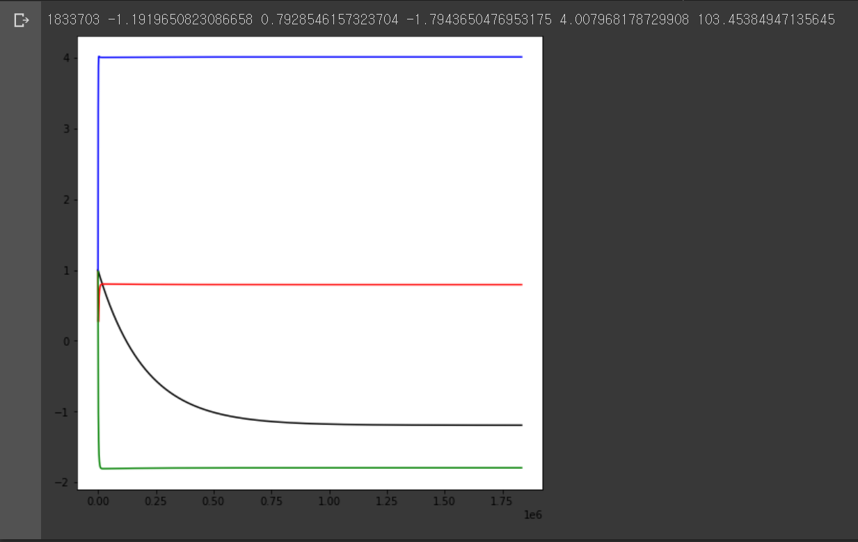

데이터 셋이 3차원 이상일 때도 위와 같이 경사하강법을 통해 선형 회귀 분석을 할 수 있다. 위 그래프는 경사하강법 각 단계에 따른 $(\theta_0, \theta_1, \theta_2, \theta_3)$의 변화 과정을 나타낸 것이다. $(\theta_0, \theta_1, \theta_2, \theta_3)$의 그래프 색은 각각 검정, 빨강, 초록, 파랑이다. $\theta_1$을 제외한 나머지 변수는 빠르게 특정 값에 수렴된 것을 볼 수 있다.

경사하강법으로 변수가 여러 개인 선형 회귀 분석을 하는 과정은 아래와 같다.

1. 4차원의(변수 4개) 데이터 셋을 불러온다. $x_i, y_i, z_i$는 입력값이고, $h_i$는 기대되는 출력값이다.
   $\{(x_i, y_i, z_i, h_i), ...\}$

2. 선형 함수(1차 함수)를 설정한다.
   $f_\theta(x, y, z) = \theta_0 + \theta_1 x + \theta_2 y+ \theta_3 z$, $where$ $\theta = (\theta_0, \theta_1, \theta_2, \theta_3)$

3. 목적 함수(에러 함수)를 설정한다. 우리는 이 목적 함수가 최소가 되게 하는 $\theta_0$, $\theta_1$, $\theta_2$, $\theta_3$을 구하려고 한다.
   $J(\theta) = \frac 1 {2m}\ \Sigma_{i=1}^m(f_\theta(x_i, y_i, z_i) - h_i)^2$, $where$ $\theta = (\theta_0, \theta_1, \theta_2, \theta_3)$

4. 경사하강법(Gradient Descent)으로 목적 함수의 값이 최소가 되는 지점의 $\theta_0$, $\theta_1$, $\theta_2$, $\theta_3$을 찾아간다. $\alpha$ 값은 너무 크면 $\theta$ 값이 발산하고, 너무 작으면 수렴하지만 계산이 오래 걸리기 때문에 적절한 값으로 설정한다.
   ${\theta_0}_{(i+1)} = {\theta_0}_i - \alpha \frac {dJ(\theta_i)} {d{\theta_0}_i}$, ${\lim\limits_{i\to\infin}{\theta_0}_i}$
   ${\theta_1}_{(i+1)} = {\theta_1}_i - \alpha \frac {dJ(\theta_i)} {d{\theta_1}_i}$, ${\lim\limits_{i\to\infin}{\theta_1}_i}$
   ${\theta_2}_{(i+1)} = {\theta_2}_i - \alpha \frac {dJ(\theta_i)} {d{\theta_2}_i}$, ${\lim\limits_{i\to\infin}{\theta_2}_i}$
   ${\theta_3}_{(i+1)} = {\theta_3}_i - \alpha \frac {dJ(\theta_i)} {d{\theta_3}_i}$, ${\lim\limits_{i\to\infin}{\theta_3}_i}$
   $where$ $\theta_i = ({\theta_0}_i, {\theta_1}_i, {\theta_2}_i, {\theta_3}_i)$

5. 경사하강법의 매 단계마다 $(\theta_0, \theta_1, \theta_2, \theta_3)$ 값을 저장해 그래프로 그린다.

2. 오차 함수 변화 표현하기

import csv
import matplotlib.pyplot as plt
from math import isclose

# Linear Model
def f(theta0, theta1, theta2, theta3, x, y, z):
  return theta0 + theta1 * x + theta2 * y + theta3 * z

# Objective Function
def J(theta0, theta1, theta2, theta3, points):
  sigma = 0
  for point in points:
    sigma += (f(theta0, theta1, theta2, theta3, point[0], point[1], point[2]) - point[3]) ** 2
  return (1 / (2 * len(points))) * sigma

# Derivative of Objective Function by theta_i
def dJ_dtheta_i(theta0, theta1, theta2, theta3, points, i):
  sigma = 0
  for point in points:
    if(i is 0):
      sigma += (f(theta0, theta1, theta2, theta3, point[0], point[1], point[2]) - point[3])
    else:
      sigma += (f(theta0, theta1, theta2, theta3, point[0], point[1], point[2]) - point[3]) * point[i - 1]
  return (1 / len(points)) * sigma


# training data set
train_set = []

# load training data set
with open('drive/My Drive/.../data_train.csv', newline='') as myfile:
  reader = csv.reader(myfile, delimiter=',')
  for i in reader:
    train_set.append([float(i[0]), float(i[1]), float(i[2]), float(i[3])])

# the initial condition
theta0 = 1
theta1 = 1
theta2 = 1
theta3 = 1
learning_rate = 0.00002
J_i = []

while(1):
  # plot the objective function at every iteration of gradient descent
  J_i.append(J(theta0, theta1, theta2, theta3, train_set))

  # the optimization is performed using the training dataset ('data_train.csv')
  next_theta0 = theta0 - learning_rate * dJ_dtheta_i(theta0, theta1, theta2, theta3, train_set, 0)
  next_theta1 = theta1 - learning_rate * dJ_dtheta_i(theta0, theta1, theta2, theta3, train_set, 1)
  next_theta2 = theta2 - learning_rate * dJ_dtheta_i(theta0, theta1, theta2, theta3, train_set, 2)
  next_theta3 = theta3 - learning_rate * dJ_dtheta_i(theta0, theta1, theta2, theta3, train_set, 3)

  # the gradient descent is performed until the convergence of (θ0, θ1, θ2, θ3) is achieved
  if(isclose(next_theta0, theta0) and isclose(next_theta1, theta1) and isclose(next_theta2, theta2) and isclose(next_theta3, theta3)):
    break

  # update {(θ0, θ1, θ2, θ3)}
  theta0 = next_theta0
  theta1 = next_theta1
  theta2 = next_theta2
  theta3 = next_theta3
  
# debug
print('Step count:', len(J_i)) 
print('Theta0:', theta0)
print('Theta1:', theta1)
print('Theta2:', theta2)
print('Theta3:', theta3)
print('J(t0, t1, t2, t3) with traning data:', J(train_set, theta0, theta1, theta2, theta3))

# plot the training error J(θ0, θ1, θ2, θ3) at every iteration of gradient descent until convergence (in blue color)
plt.figure(figsize=(8, 8))
plt.plot(range(len(J_i)), J_i, color='blue')
plt.show()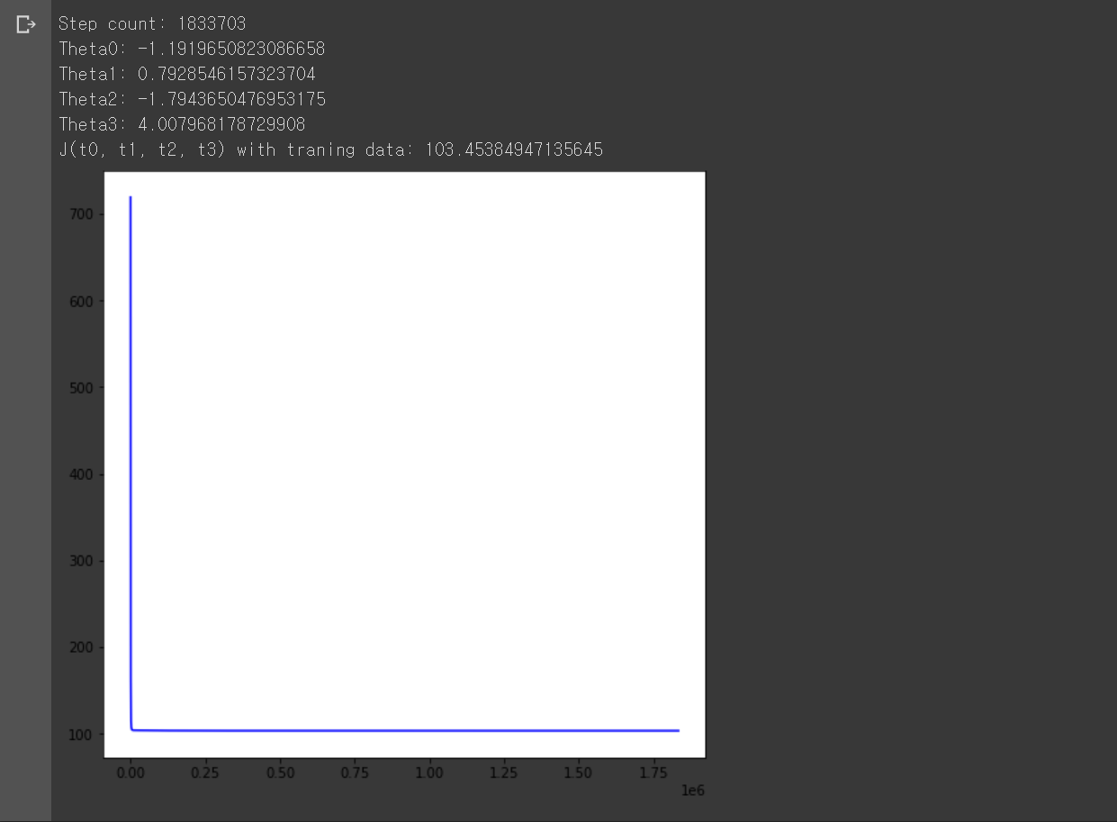

위 코드랑 거의 동일하고, 출력 그래프만 매 경사하강법 단계마다 목적 함수가 어떻게 변경되는지로 변경됐다. 목적 함수가 수렴하는 것에 비해 반복 횟수가 너무 많아 그래프의 변화가 잘 보이지 않는다.