[Review] Fourier Features Let Networks Learn High-Frequency Functions in Low Dimensional Domains
3D AI
이 논문은 Neural Tangent Kernel 을 바탕으로 Fourier-featuring (coordinate space point 의 frequency space 로의 embedding) 이 network 관점에서 stationary 한 (isotrophic) 성질을 갖게 된다는 사실을 수학적으로 규명하고, 이를 통해 3d shape, 2d reconstruction 등의 low-dimension to high-dimension vision task 의 성능을 증대시킬 수 있다는 것을 이론적, 실험적으로 규명한 논문이다.
NeurIPS2020 Spotlight
1. Introduction
Fourier-featuring 이란, coordinate space point 를 frequency space 로 embedding 하는 function 의 총칭 이다.
Deeplearning model 에서의 대표적인 예시로는, Transformer architecture model 들이 attention 만으로는 원본 위치 정보를 알 수 없으므로, feature 의 위치 정보를 포함시키기 위해 sinusoidal function 을 통해 coordinate space 에서 frequency space 로의 embedding 을 진행하는 'Positional Encoding' 등이 있다.
위 논문은 NTK theory 를 통해
- fourier-featuring 을 통해 neural network 가 coordinate information 을 어떻게 받아들이게 되는지 이론적으로 규명하고,
- 다양한 Vision task 에서 이를 활용한 qualitative case 를 제시하였다.
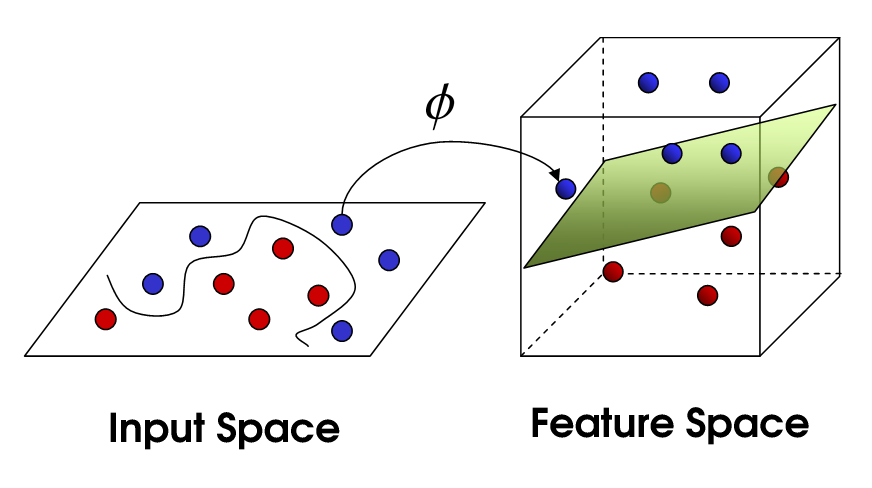
저자들은 또한 다음 그림과 같이,
.png)
- Dense 하고 continuous & uniform 한 low-dimension data input
- high-dimensional output
을 모두 만족하는 neural network를 coordinate-based MLP 라고 명명한다.
이 논문을 이해하기 위해 kernel trick 과 neural tangent kernel 에 대한 이해가 필요하므로, 간단하게 서술하고 넘어가도록 하겠다.
2. Preliminaries
2.1. Kernel Trick
Linearly inseparable 한 data point 에 대하여 (: feature map) 는 linear separability 를 갖게 만드는 non-linear mapping function 이라 하자.
이때 kernel trick 은 이러한 feature map 을 explicit 하게 구하지 않고, kernel 을 통해서 feature space 를 구하는 kernel regression 이며, 다음과 같이 정의한다.
이는 input 에 feature mapping 을 거친 후에 내적을 취해준다기 보단, kernel 을 통해 좋은 성질을 갖는 feature map 를 구할 수 있다고 해석하는 편이 좋다.
2.2. Neural Tangent Kernel (NeurIPS2018)
Neural tangent kernel 은, 이러한 kernel trick 을 이용해 neural network 를 설명하려는 노력의 일환으로, width 가 무한대인 deep한 NN의 GD based training 을 kernel regression 으로 설명하는 이론이다.
2.2.1. Linearization of NN training & Kernel Definition
어떠한 neural network model 을 위와 같은 linearization 으로 표현할 수 있다. 이때 Taylor expanded tangent line 은 다음과 같은 성질을 가지는데,
- weight 에 대해서 linear
- 에 대해서 non-linear
이에 따라 tangent line 의 gradient term 을 다음과 같이 해석할 수 있다.
- : non-linear data point 를 어떠한 유용한 space 에 mapping 하는 feature map.
이에 해당하는 kernel 는 다음과 같이 정의할 수 있다.
2.2.2. Gradient-based Training & Kernel Regression
이때, 정의된 neural tangent kernel 을 neural network 의 gradient descent 에서 찾을 수 있다. timestep 에 대하여 gradient descent 를 다음과 같이 표현해보자.
이제 least square (MSE) 이 loss function 일 때, 다음과 같이 를 구할 수 있고,
이에 따라 optimization-based neural network training 을 다음과 같이 NTK kernel regression 으로 나타낼 수 있다.
이제 라고 하자. 이 때, training iteration 에서의 output residual 을 다음과 같이 표현할 수 있다.
2.3. Spectral Bias of DNNs
이제 논문에서의 Eq.3 을 자세히 살펴보겠다.
위 절에서 살펴 보았던 NTK approximation 에 따라, test data 에 대해 iteration 이후의 network 의 prediction 은 다음과 같이 표현할 수 있다.
이상적인 training 에 대해서 가 성립할 것이기 때문에, 2.2.2 마지막 eq 의 residual 을 통해 output 을 표현한 것과 같은 형태임을 알 수 있다.
이제 우리는 NTK kernel 를 eigendecomposition 하여 로 나타낼 때, 위 식을 다음과 같이 표현할 수 있다.
따라서 우리는 exponential 의 지수 항이 eigenvalue 값에 따라 decay 됨을 알 수 있고, 이는 즉 larger eigenvalue 가 먼저 빨리 배우게 됨을 의미한다.
이미지 fourier transform 에서 large eigenvalue 는 전체적인 image 의 contour 등을 담당하고 있으므로, high frequency component 에 대한 convergence 가 느릴 것이다. 이는 NeRF 에서 embedding 을 적용하지 않을 시 fine detail 에 대한 convergence 가 매우 느린 것을 수학적으로 규명한다.
3. Fourier Features for a Tunable Stationary Neural Tangent Kernel
이 절에서 저자들은 Fourier Features Embedding 이 Kernel space 상에서 어떠한 역할을 하는지 규명하고, 이를 통해 High frequency component 에 대한 convergence 를 어떻게 효과적으로 다루는지에 대해 설명한다.
3.1. Fourier-Feature Mapping & Kernel Regression
3.1.1. Fourier-Feature Mapping
Fourier-Feature mapping function 를 다음과 같이 정의할 수 있다.
-
e.g. Positional Encoding in Transformer :
Transformer 등의 attention-based architecture 에서 spatial information 을 feature 에 더해주기 위한 encoding 방식이며, 다음과 같이 정의된다.
-
e.g. Positional Encoding in NeRF :
Coordinate-based MLP 에서 network input 이 low/high frequency information 을 골고루 잘 포함할 수 있도록 하는 encoding 이며, 다음과 같이 정의된다.
3.1.2. Kernel Regression to Fourier-Feature mapping
우리는 이 mapping function 으로부터 induced 되는 kernel 을 다음과 같이 정의할 수 있으며, 으로부터
fourier featuring kernel 이 2개의 input coordinates 에 대한 stationary function 으로 표현됨을 알 수 있다.
- stationary function 은 translation-invariant 한 특성을 갖는 function 을 의미한다. 여기서는 이기 때문에 stationary 한 성질을 만족한다.
Cooridnate-based MLP는 dense & uniform coordinate points 를 입력으로 받아 정보를 추출하는데, global 하게 좋은 성능을 내기 위해서는 isotropic 해야한다. 이는 특정 방향이 아닌, 전방위적으로 feature 를 추출해야하기 때문이다.
- 따라서 location 에 상관없이 modeling 을 진행할 수 있는 stationary 성질이 갖춰졌을 때 좋은 성능을 기대할 수 있다.
- 이는 image positional encoding 이 원래 coordinate system 에서 같은 거리만큼 떨어져 있는 관계는 위치 정보에 따른 weight 를 모두 같게 처리하기 때문이며, 좌표의 relative relation 을 high-dimensional space 에서 복각할 수 있다는 것.
3.2. NTK Kernel with Fourier-Featuring
이제 NTK fourier-featured kernel 을 다음과 같이 쓸 수 있다.
- 여기서 stationary kernel regression 은 convolutional filter 를 통한 reconstruction 과 같음을 알 수 있다. neural network 가 data point 와 이에 대한 weight 에서 와 의 합성 kernel 사이의 convolution 을 approximate 하기 때문.
따라서 NTK theory 을 통해 나타낸 fourier featuring 은 최종적으로 다음과 같다.
여기서 는 direc delta 이다. 위 식의 의미를 다음과 같이 해석할 수 있다.
- Stationary 한 filter 를 통해 coordinate system 상에서의 정보를 location-invariant 하게 추출한다.
- Convolution 은 frequency space 에서 multiplication 의 IFT 이기 때문에, 에서 직접적으로 embedding 된 특정 frequency 의 componenet 들을 통해 서로 다른 frequency space 에서의 feature 를 다각도로 (그러나 location invariant 하게) 얻을 수 있다.
- Fourier-featured input 을 입력받는 NN 은 NTK 와 어떤 stationary kernel 을 합성해서 kernel regression 을 수행하는 것과 같다.
4. Experiments
.png)
.png)
You may also likes:

잘 정리해주셔서 큰 도움이 됐습니다.
아래 부분에 오타가 있는 것 같아서 댓글 남겨요
2.2.1. Linearization of NN training & Kernel Definition
의 커널을 정리하는 맨 마지막 수식에서 {ϕ(x)^T, ϕ(x')} 가 되어야 할 것 같은데 한번 확인 부탁 드려요!
감사합니다.