Lec7: Numerical Python - Numpy
- 코드로 방정식 표현
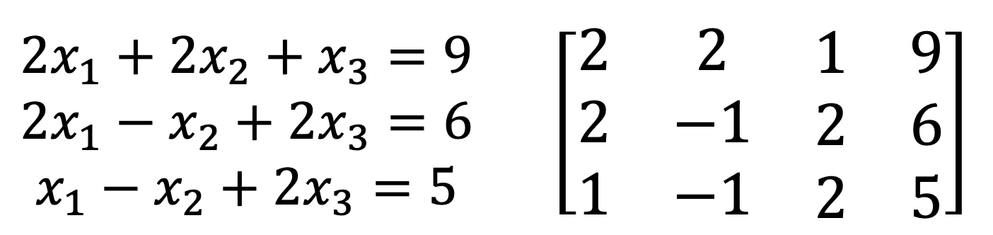
coefficient_matrix = [[2, 2, 1], [2, -1, 2], [1, -1, 2]]
constant_vector = [9, 6, 5]- 다양한 Matrix 계산을 어떻게 만들 것인가?
- 굉장히 큰 Matrix에 대한 표현
- 처리 속도 문제 : Python은 Interpreter Language
적절한 Package의 활용이 필요 : Numpy
01_Python Science Process Package : Numpy
1) Numpy
- Numerical Python
- Python의 고성능 과학 계산용 Package
- Matrix와 Vector와 같은 Array 연산의 표준
특징
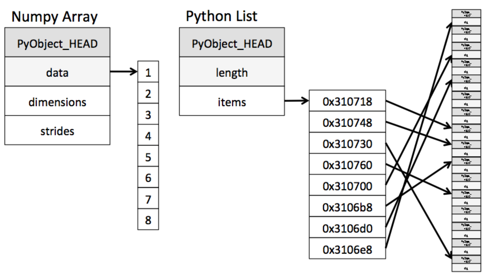
- 일반 List에 비해 빠르고, 메모리 효율적
- 반복문 없이 Data Array에 대한 처리를 지원
- 선형대수와 관련된 다양한 기능을 제공
- C, C++, 포트란 등의 언어와 통합 가능
2) ndarray : N-Dimension Array
- Numpy의 호출 방법
- 일반적으로 np라는 alias 이용해서 호출
import numpy as np3) Array Creation
test_array = np.array([1, 4, 5, 8], float)
print(test_array) # array([1. 4. 5. 8.])
type(test_array[3]) # numpy.float64- Numpy는 np.array Function으로 Array 생성
- Numpy는 하나의 Data Type만 Array에 넣을 수 있음
- List와 가장 큰 차이점 : Dynamic Typing not Supported
- C의 Array를 사용하여 Array 생성
- Shape : Numpy Array의 Dimension 구성을 Return
- Dtype : Numpy Array의 Data Type을 Return
test_array = np.array([1, 4, 5, "8"], float) # String Type의 데이터를 입력해도
print(test_array)
print(type(test_array[3])) # Float Type으로 자동 형변환을 실시
print(test_array.dtype) # Array 전체의 데이터 Type을 Return
print(test_array.shape) # Array의 shape을 Return[1. 4. 5. 8.]
<class 'numpy.float64'>
float64
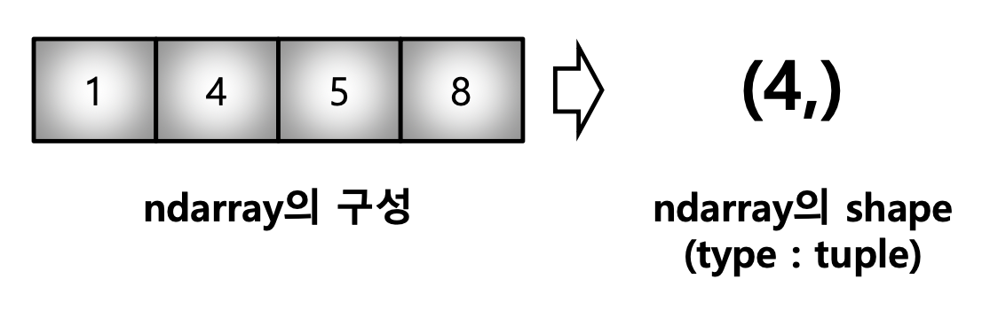
(4,)4) Array Shape
- Array의 RANK에 따라 불리는 이름이 존재
- Shape = Array의 크기, 형태 등에 대한 정보
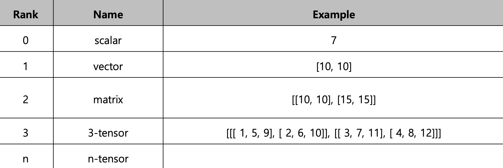
- Vector
- Matrix
matrix = [[1, 2, 5, 8], [1, 2, 5, 8], [1, 2, 5, 8]]
np.array(matrix, int).shape # (3, 4)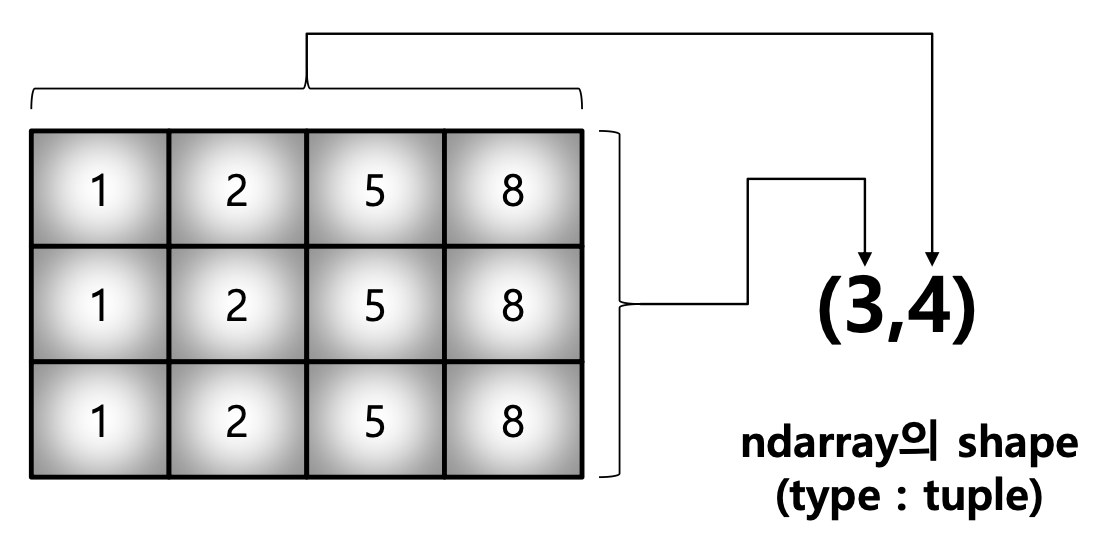
- 3rd Order Tensor
1) ndim : Number of Dimensions
2) size : Data의 개수
tensor = [[[1, 2, 5, 8], [1, 2, 5, 8], [1, 2, 5, 8]],
          [[1, 2, 5, 8], [1, 2, 5, 8], [1, 2, 5, 8]],
          [[1, 2, 5, 8], [1, 2, 5, 8], [1, 2, 5, 8]],
          [[1, 2, 5, 8], [1, 2, 5, 8], [1, 2, 5, 8]]]
np.array(tensor, int).shape
# (4, 3, 4)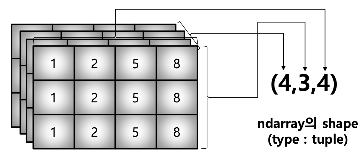
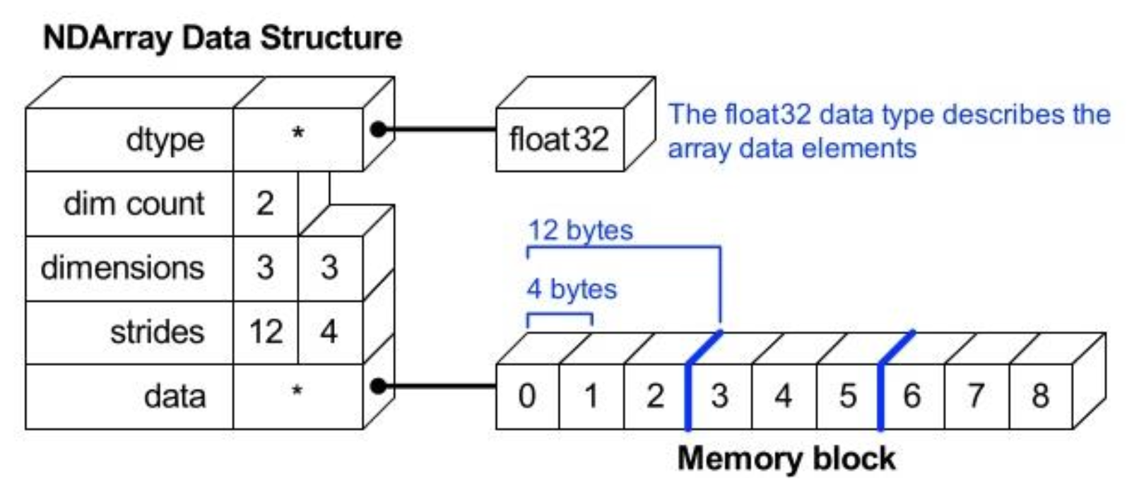
5) Array Dtype
- ndarray의 Single Element가 가지는 Data Type
- 각 Element가 차지하는 Memory의 크기가 결정됨
np.array([[1, 2, 3], [4.5, 5, 6]], dtype=int) # Data Type을 integer로 선언
# array([[1, 2, 3],
#        [4, 5, 6]])

np.array([[1, 2, 3], [4.5, "5", "6"]], dtype=np.float32) # Data Type을 float로 선언
# array([[1. , 2. , 3. ],
# [4.5, 5. , 6. ]], dtype=float32)- C의 Data Type과 Compatible
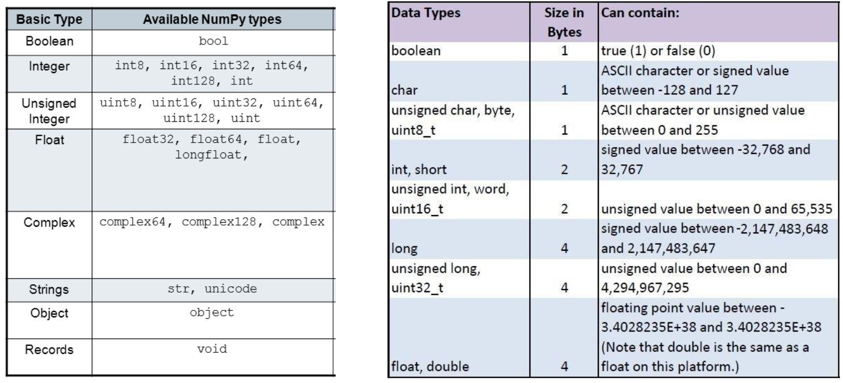
6) Array nbytes
nbytes : ndarray Object의 Memory Size를 Return
np.array([[1, 2, 3], [4.5, "5", "6"]], dtype=np.float32).nbytes # 32 = 4bytes, 6 * 4bytes = 24
np.array([[1, 2, 3], [4.5, "5", "6"]], dtype=np.int8).nbytes # 6
np.array([[1, 2, 3], [4.5, "5", "6"]], dtype=np.float64).nbytes # 48
02_Handling Shape
1) Reshape
Reshape : Array의 Shape의 크기를 변경, Element의 갯수는 동일, Return은 없음.
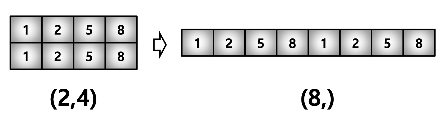
test_matrix = [[1, 2, 3, 4], [1, 2, 5, 8]]
np.array(test_matrix).shape # (2, 4)
np.array(test_matrix).reshape(8,) # array([1, 2, 3, 4, 1, 2, 5, 8])
np.array(test_matrix).reshape(8,).shape # (8,)np.array(test_matrix).reshape(2, 4).shape # (2, 4)
np.array(test_matrix).reshape(-1, 2).shape # (4, 2)
# -1: size를 기반으로 row 개수 선정
np.array(test_matrix).reshape(2, 2, 2)
# array([[[1, 2],
# [3, 4]],
#
# [[1, 2],
# [5, 8]]])
np.array(test_matrix).reshape(2, 2, 2).shape # (2, 2, 2)2) Flatten : N-Dimension Array를 1차원 Array로 변환
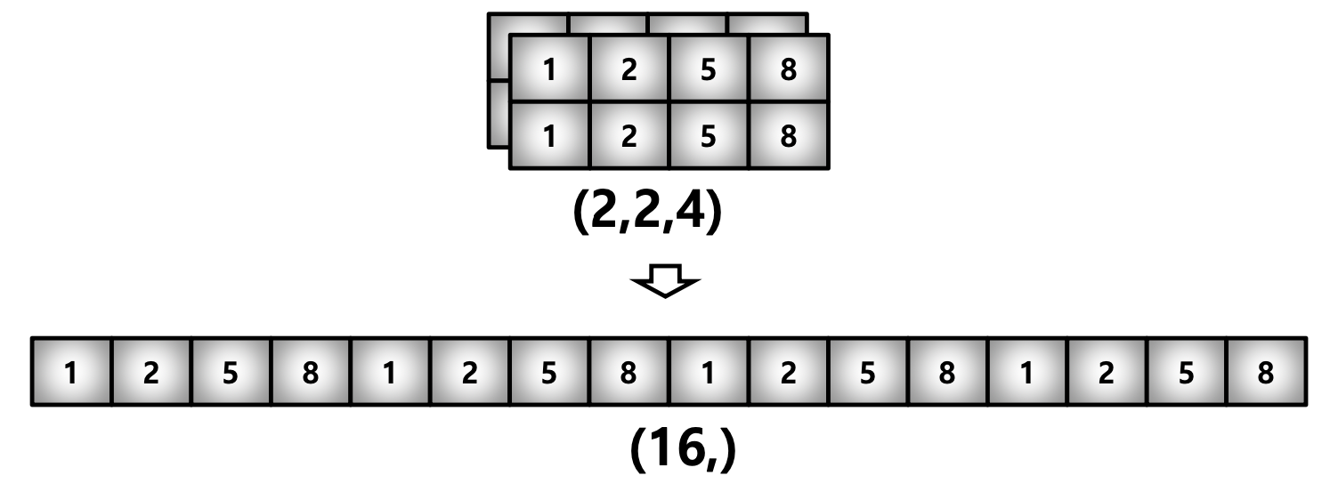
test_matrix = [[[1, 2, 3, 4], [1, 2, 5, 8]], [[1, 2, 3, 4], [1, 2, 5, 8]]]
np.array(test_matrix).flatten()
# array([1, 2, 3, 4, 1, 2, 5, 8, 1, 2, 3, 4, 1, 2, 5, 8])
03_Indexing & Slicing
1) Indexing for Numpy Array
- List와 달리 2차원 Array에서 [0, 0] 표기법을 제공
- Matrix일 경우 앞은 Row, 뒤는 Column을 의미
a = np.array([[1, 2, 3], [4.5, 5, 6]], int)
print(a)
# [[1 2 3]
#  [4 5 6]]
print(a[0,0]) # Two dimensional array representation #1
# 1
print(a[0][0]) # Two dimensional array representation #2
# 1

a[0,0] = 12 # Matrix 0,0 에 12 할당
print(a)
# [[12  2  3]
#  [ 4  5  6]]
a[0][0] = 5 # Matrix 0,0 에 12 할당
print(a)
# [[5 2 3]
#  [4 5 6]]
2) Slicing for Numpy Array
- List와 달리 Row와 Column 부분을 나눠서 Slicing이 가능함
- Matrix의 부분 집합을 추출할 때 유용
import numpy as np
matrix = np.array([[1, 2, 3],
[4, 5 ,6],
[7, 8, 9]])
# matrix[row_start:row_stop:row_step, col_start:col_stop:col_step]
row = matrix[1, :] # 2번 행, 열 전부
print(row)
# [4 5 6]
col = matrix[:, 0] # 행 전부, 1번 열
print(col)
# [1 4 7]
submatrix = matrix[:2, :2] # 1 ~ 2행, 1 ~ 2열
print(submatrix)
# [[1 2]
# [4 5]]
middle_rows = matrix[1:, :] # 2 ~ 3행, 열 전부
print(middle_rows)
# [[4 5 6]
# [7 8 9]]
middle_cols = matrix[:, 1:] # 행 전부, 2 ~ 3열
print(middle_cols)
# [[2 3]
# [5 6]
# [8 9]]
submatrix2 = matrix[0:2, 1:] # 1 ~ 2행, 2 ~ 3열
print(submatrix2)
# [[2 3]
# [5 6]]
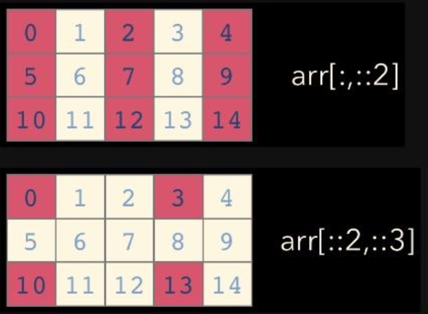
step_matrix = matrix[::2, ::2] # 1 ~ 3행(두칸씩), 1 ~ 3열(두칸씩)
print(step_matrix)
# [[1 3]
# [7 9]]import numpy as np
tensor = np.array([[[1, 2, 3, 4],
[5, 6, 7, 8],
[9, 10, 11, 12]],
[[13, 14, 15, 16],
[17, 18, 19, 20],
[21, 22, 23, 24]]])
# tensor[depth_start:depth_stop:depth_step, row_start:row_stop:row_step, col_start:col_stop:col_step]
matrix = tensor[0, :, :] # 1번 2D Array 선택
print(matrix)
# [[1 2 3 4]
# [5 6 7 8]
# [9 10 11 12]]
sliced_tensor = tensor[:, 1:3, 1:] # 모든 2D Array, 2 ~ 3행, 2 ~ 4열
print(sliced_tensor)
# [[[6 7 8]
# [10 11 12]]
#
# [[18 19 20]
# [22 23 24]]]
step_tensor = tensor[::, 1:3, 1::2] # 모든 2D Array, 2 ~ 3행, 2 ~ 4열(2칸씩)
print(step_tensor)
# [[[ 6 8]
# [10 12]]
#
# [[18 20]
# [22 24]]]04_Creation Function
1) Arange
- Array Range를 지정하여, 값의 List를 생성하는 명령어
import numpy as np

np.arange(30) # range : List의 range와 같은 효과, integer로 0부터 29까지 배열 추출array([ 0, 1, 2, 3, 4, 5, 6, 7, 8, 9, 10, 11, 12, 13, 14, 15, 16, 17, 18, 19, 20, 21, 22, 23, 24, 25, 26, 27, 28, 29])
np.arange(0, 5, 0.5) # Floating Point도 표시 가능array([0. , 0.5, 1. , 1.5, 2. , 2.5, 3. , 3.5, 4. , 4.5])
np.arange(30).reshape(5, 6)array([[ 0, 1, 2, 3, 4, 5], [ 6, 7, 8, 9, 10, 11], [12, 13, 14, 15, 16, 17], [18, 19, 20, 21, 22, 23], [24, 25, 26, 27, 28, 29]])
2) Ones, Zeros and Empty
- zeros : 0으로 가득찬 ndarray 생성
# np.zeros(shape, dtype, order)
np.zeros(shape=(10,), dtype=np.int8) # 10 zero vector 생성array([0, 0, 0, 0, 0, 0, 0, 0, 0, 0], dtype=int8)
np.zeros((2, 5)) # 2 by 5 zero matrix 생성array([[0., 0., 0., 0., 0.], [0., 0., 0., 0., 0.]])
- ones : 1로 가득찬 ndarray 생성
# np.ones(shape, dtype, order)
np.ones(shape=(10,), dtype=np.int8)array([1, 1, 1, 1, 1, 1, 1, 1, 1, 1], dtype=int8)
np.ones((2, 5))array([[1., 1., 1., 1., 1.], [1., 1., 1., 1., 1.]])
- empty : shape만 주어지고 비어있는 ndarray 생성,
Memory Initialization이 되지 않기 때문에 실행 마다 값이 변한다.
np.empty(shape=(10,), dtype=np.int8)array([0, 0, 0, 0, 0, 0, 0, 0, 0, 0], dtype=int8)
np.empty((3, 5))array([[0. , 0. , 0.4472136 , 0.0531494 , 0.18257419], [0.4472136 , 0.2125976 , 0.36514837, 0.4472136 , 0.4783446 ], [0.54772256, 0.4472136 , 0.85039041, 0.73029674, 0.4472136 ]])
3) Something_like
- 기존 ndarray의 shape 크기 만큼 1, 0 또는 empty array를 Return
test_matrix = np.arange(30).reshape(5, 6)
np.ones_like(test_matrix)array([[1, 1, 1, 1, 1, 1], [1, 1, 1, 1, 1, 1], [1, 1, 1, 1, 1, 1], [1, 1, 1, 1, 1, 1], [1, 1, 1, 1, 1, 1]])
4) Identity
- 단위 행렬(i Matrix)를 생성
# n : Number of Rows
np.identity(n=3, dtype=np.int8)array([[1, 0, 0], [0, 1, 0], [0, 0, 1]], dtype=int8)
np.identity(5)array([[1., 0., 0., 0., 0.], [0., 1., 0., 0., 0.], [0., 0., 1., 0., 0.], [0., 0., 0., 1., 0.], [0., 0., 0., 0., 1.]])
5) Eye
- 대각선이 1인 Matrix, k값의 시작 index의 변경이 가능
np.eye(3, 5)array([[1., 0., 0., 0., 0.], [0., 1., 0., 0., 0.], [0., 0., 1., 0., 0.]])
np.eye(3, 5, k=2)array([[0., 0., 1., 0., 0.], [0., 0., 0., 1., 0.], [0., 0., 0., 0., 1.]])
np.eye(N=3, M=5, dtype=np.int8)array([[1, 0, 0, 0, 0], [0, 1, 0, 0, 0], [0, 0, 1, 0, 0]], dtype=int8)
6) Diag
- 대각 Matrix의 값을 추출
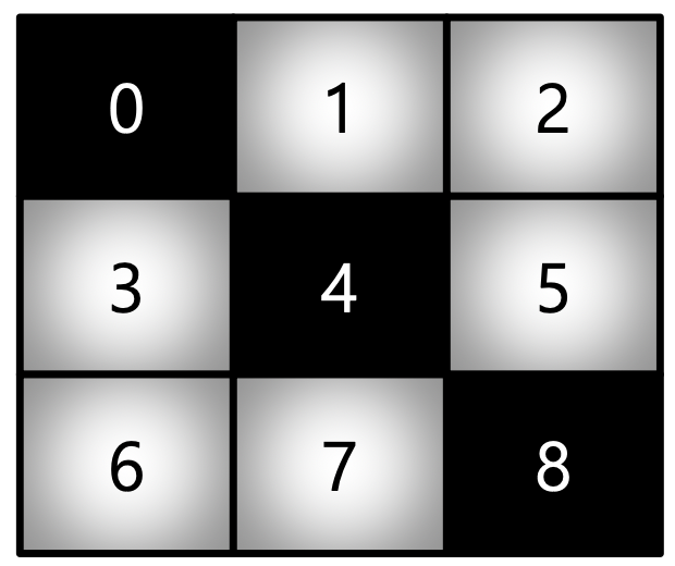
matrix = np.arange(9).reshape(3, 3)
np.diag(matrix)array([0, 4, 8])
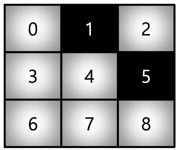
# k : Start Index
np.diag(matrix, k=1)array([1, 5])
7) Random Sampling
- Data 분포에 따른 Sampling으로 Array를 생성
np.random.uniform(0, 1, 10).reshape(2, 5) # 균등 분포array([[0.70092722, 0.81758067, 0.39107449, 0.36800408, 0.8886006 ], [0.44608869, 0.39946623, 0.48868277, 0.56322106, 0.39963681]])
np.random.normal(0, 1, 10).reshape(2, 5) # 정규 분포array([[-0.08111845, -2.73108964, -1.21516222, 0.05078398, 0.48177804], [ 1.21849554, -1.02722083, -1.72743057, 0.55792697, 0.31990059]])
05_Operation Functions
1) Sum
- ndarray의 Element들 간의 합을 구함, List의 Sum 기능과 동일
import numpy as np

test_array = np.arange(1, 11)
print(test_array)
test_array.sum(dtype=np.float64)
[ 1 2 3 4 5 6 7 8 9 10]
55.02) Axis
- 모든 Operation Function을 실행할 때 기준이 되는 Dimension Axis
- 새로 생성된 Axis가 Index=0
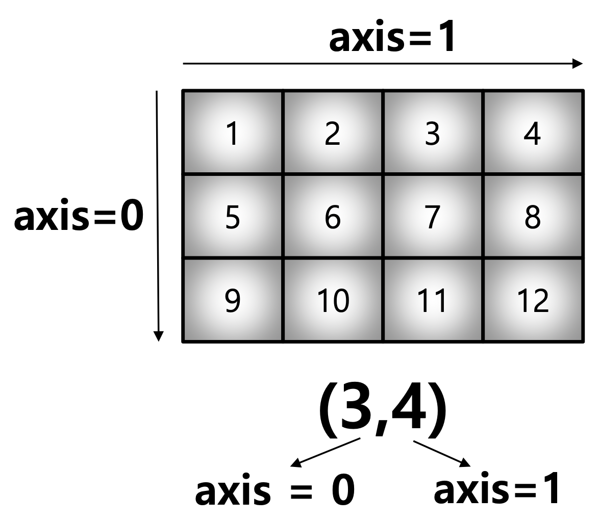
test_array = np.arange(1, 13).reshape(3, 4)
print(test_array)
test_array.sum(axis=1), test_array.sum(axis=0)[[ 1 2 3 4]
[ 5 6 7 8]
[ 9 10 11 12]]
(array([10, 26, 42]), array([15, 18, 21, 24]))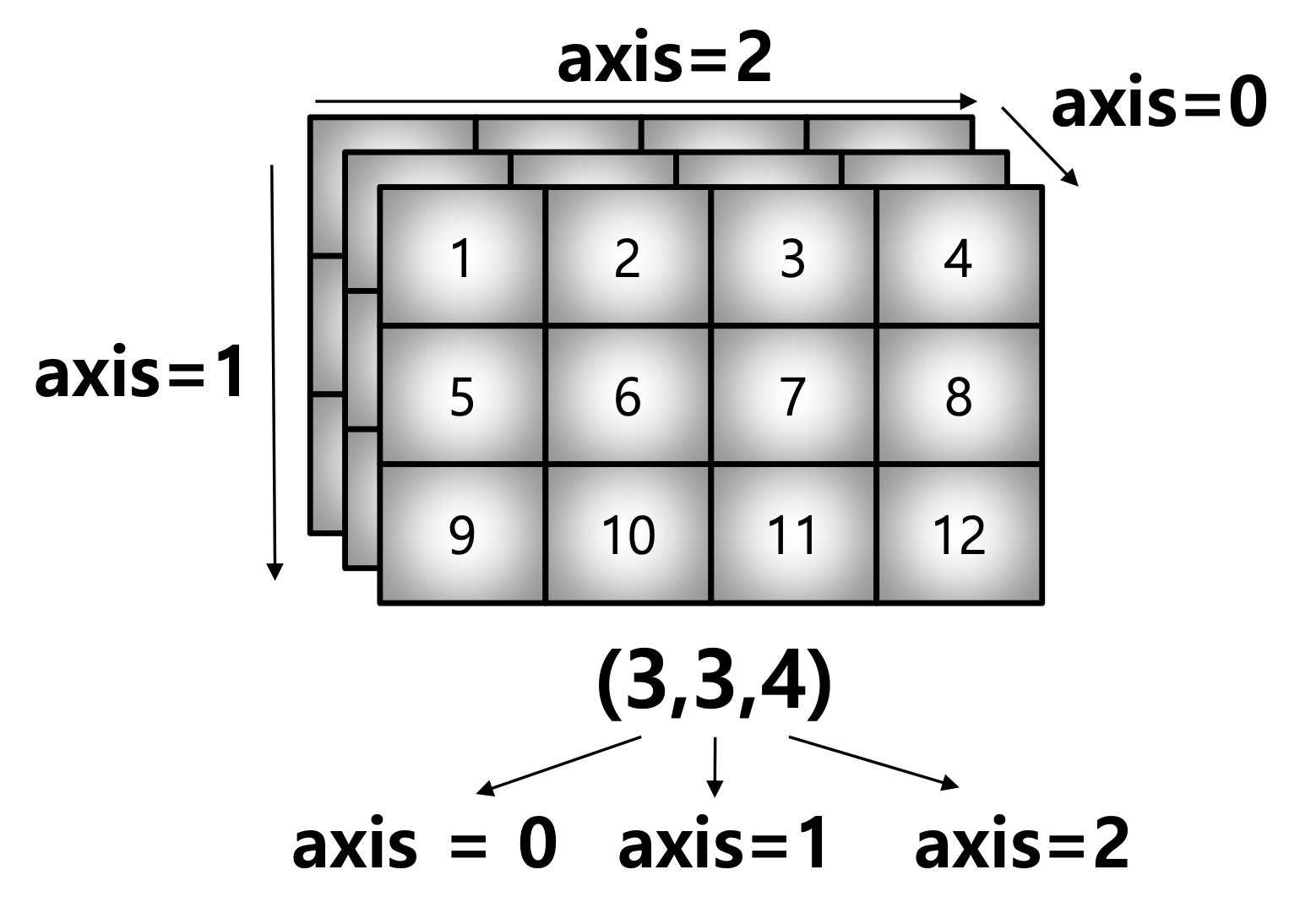
third_order_tensor = np.tile(np.arange(1, 13).reshape(3, 4), (3, 1, 1))
print(third_order_tensor)
third_order_tensor.sum(axis=2)
third_order_tensor.sum(axis=1)
third_order_tensor.sum(axis=0)[[[ 1 2 3 4]
[ 5 6 7 8]
[ 9 10 11 12]]
[[ 1 2 3 4]
[ 5 6 7 8]
[ 9 10 11 12]]
[[ 1 2 3 4]
[ 5 6 7 8]
[ 9 10 11 12]]]
array([[10, 26, 42],
[10, 26, 42],
[10, 26, 42]])
array([[15, 18, 21, 24],
[15, 18, 21, 24],
[15, 18, 21, 24]])
array([[ 3, 6, 9, 12],
[15, 18, 21, 24],
[27, 30, 33, 36]])3) Mean & Std
- ndarray의 Element들 간의 평균 또는 표준 편차를 Return
test_array = np.arange(1, 13).reshape(3, 4)
print(test_array)
test_array.mean(), test_array.mean(axis=0)
test_array.std(), test_array.std(axis=0)[[ 1 2 3 4]
[ 5 6 7 8]
[ 9 10 11 12]]
(6.5, array([5., 6., 7., 8.]))
(3.452052529534663, array([3.26598632, 3.26598632, 3.26598632, 3.26598632]))4) Mathematical Functions
- 그 외에도 다양한 수학 연산자를 제공함(np.something 호출)
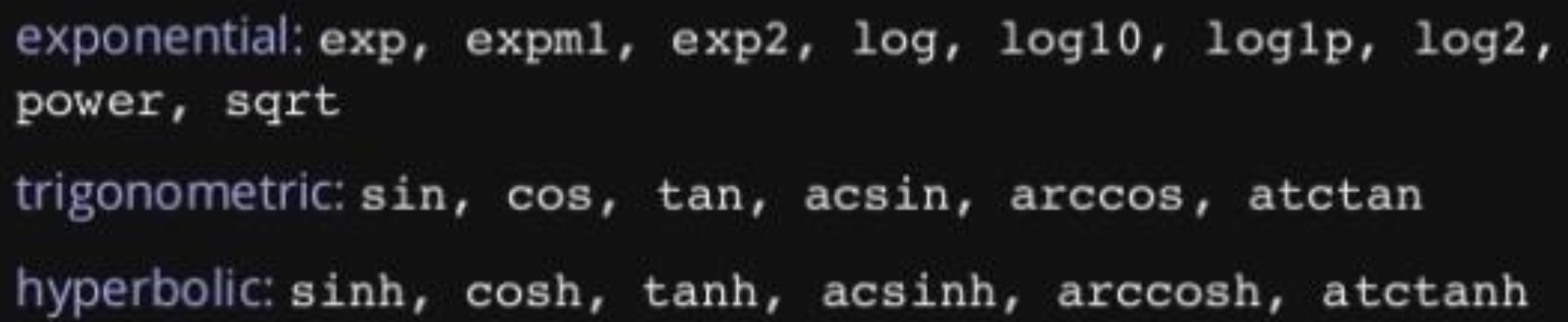
np.exp(test_array), np.sqrt(test_array)(array([[2.71828183e+00, 7.38905610e+00, 2.00855369e+01, 5.45981500e+01],
[1.48413159e+02, 4.03428793e+02, 1.09663316e+03, 2.98095799e+03],
[8.10308393e+03, 2.20264658e+04, 5.98741417e+04, 1.62754791e+05]]),
array([[1. , 1.41421356, 1.73205081, 2. ],
[2.23606798, 2.44948974, 2.64575131, 2.82842712],
[3. , 3.16227766, 3.31662479, 3.46410162]]))5) Concatenate
- Numpy Array를 합치는 Function
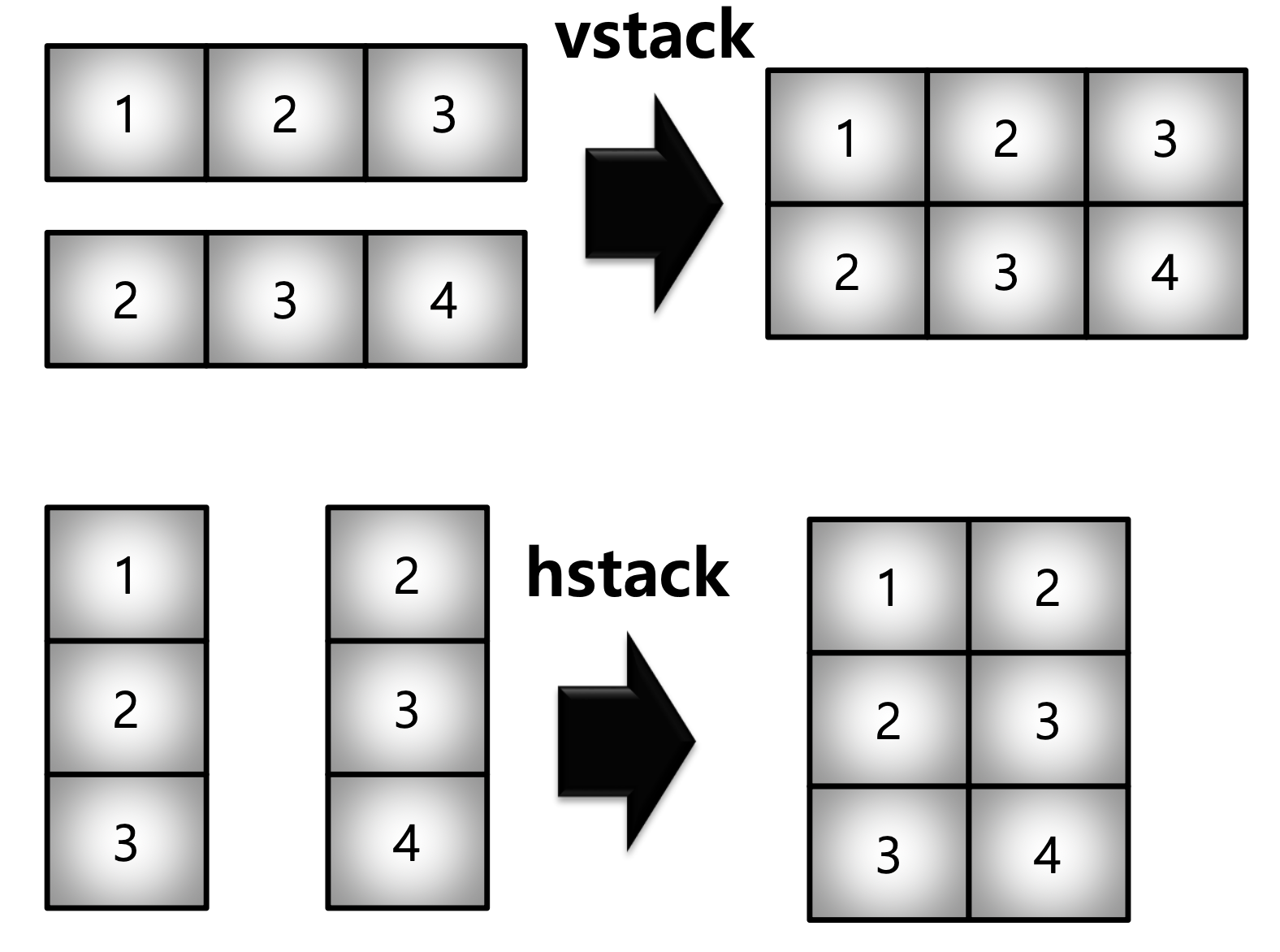
a = np.array([1, 2, 3])
b = np.array([2, 3, 4])
np.vstack((a, b))

a = np.array([ [1], [2], [3]])
b = np.array([ [2], [3], [4]])
np.hstack((a, b))array([[1, 2, 3],
[2, 3, 4]])
array([[1, 2],
[2, 3],
[3, 4]])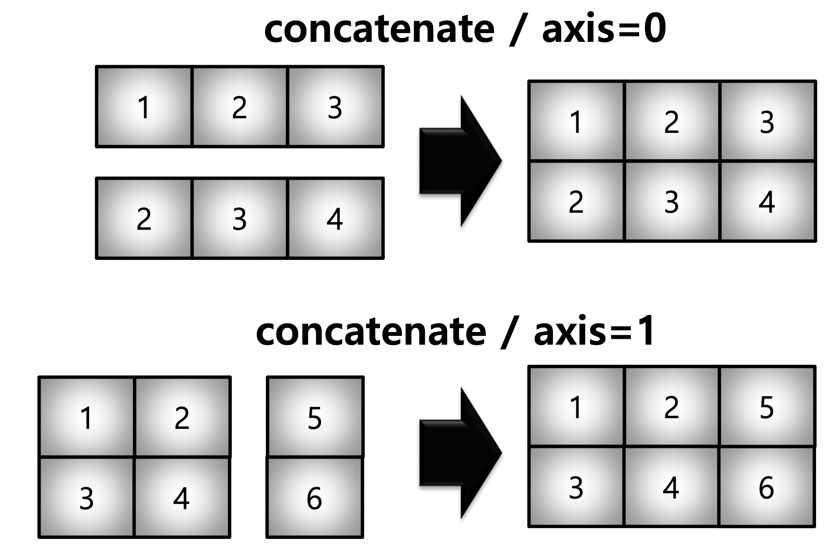
a = np.array([[1, 2, 3]])
b = np.array([[2, 3, 4]])
np.concatenate((a, b), axis=0)

a = np.array([[1, 2], [3, 4]])
b = np.array([[5, 6]])
np.concatenate((a, b.T), axis=1)array([[1, 2, 3],
[2, 3, 4]])
array([[1, 2, 5],
[3, 4, 6]])06_Array Operations
1) Operations b/t Arrays
- Numpy는 Array간의 기본적인 사칙 연산을 지원
test_a = np.array([[1, 2, 3], [4, 5, 6]], float)
test_a + test_a # Matrix + Matrix 연산
test_a - test_a # Matrix - Matrix 연산
test_a * test_a # Matrix 안의 Element들 간 같은 위치에 있는 값들끼리 연산array([[ 2., 4., 6.],
[ 8., 10., 12.]])
array([[0., 0., 0.],
[0., 0., 0.]])
array([[ 1., 4., 9.],
[16., 25., 36.]])2) Element-wise Operations
- Array 간 Shape이 같을 때 일어나는 연산
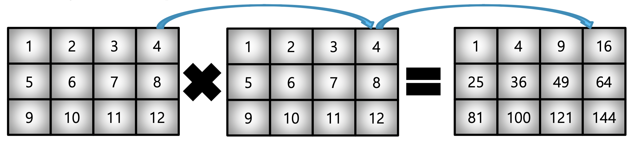
matrix_a = np.arange(1, 13).reshape(3, 4)
matrix_a * matrix_aarray([[ 1, 4, 9, 16],
[ 25, 36, 49, 64],
[ 81, 100, 121, 144]])3) Dot Product
- Matrix의 기본 연산, dot Function 사용
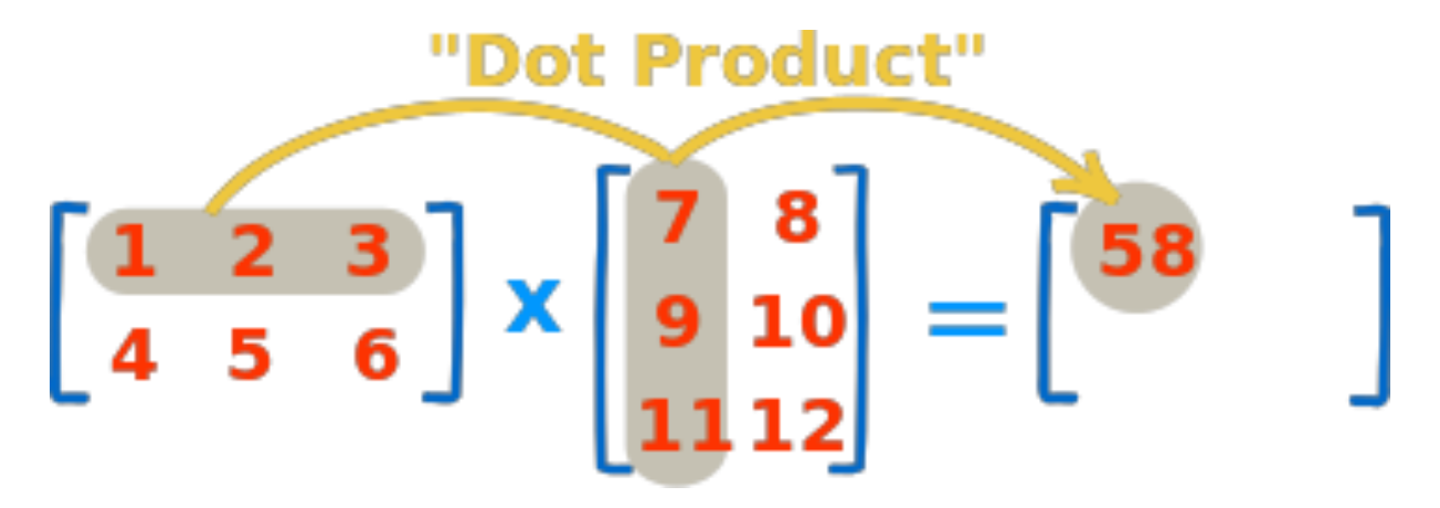
test_a = np.arange(1, 7).reshape(2, 3)
test_b = np.arange(7, 13).reshape(3, 2)
test_a.dot(test_b)array([[ 58, 64],
[139, 154]])4) Transpose
- Tranpose 또는 T Attribute 사용
test_a = np.arange(1, 7).reshape(2, 3)
print(test_a)
test_a.transpose()
test_a.T
test_a.T.dot(test_a) # Matrix 간 곱셈[[1 2 3]
[4 5 6]]
array([[1, 4],
[2, 5],
[3, 6]])
array([[1, 4],
[2, 5],
[3, 6]])
array([[17, 22, 27],
[22, 29, 36],
[27, 36, 45]])5) BroadCasting
- Shape이 다른 Array 간 연산을 지원하는 기능
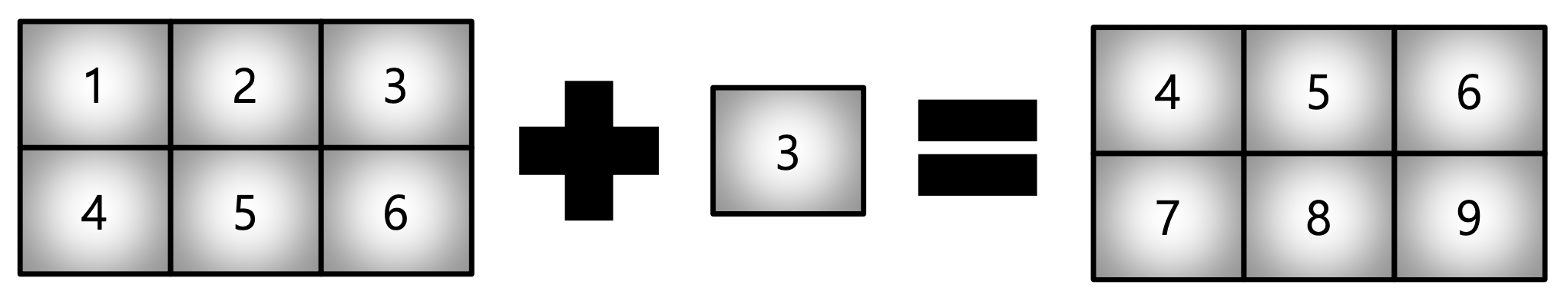
test_matrix = np.array([[1, 2, 3], [4, 5, 6]])
scalar = 3
test_matrix + scalararray([[4, 5, 6],
[7, 8, 9]])test_matrix - scalar
test_matrix * 5
test_matrix / 5
test_matrix // 0.2
test_matrix ** 2array([[-2, -1, 0],
[ 1, 2, 3]])
array([[ 5, 10, 15],
[20, 25, 30]])
array([[0.2, 0.4, 0.6],
[0.8, 1. , 1.2]])
array([[ 4., 9., 14.],
[19., 24., 29.]])
array([[ 1, 4, 9],
[16, 25, 36]])- Scalar & Vector 외에도 Vector & Matrix 간의 연산도 지원
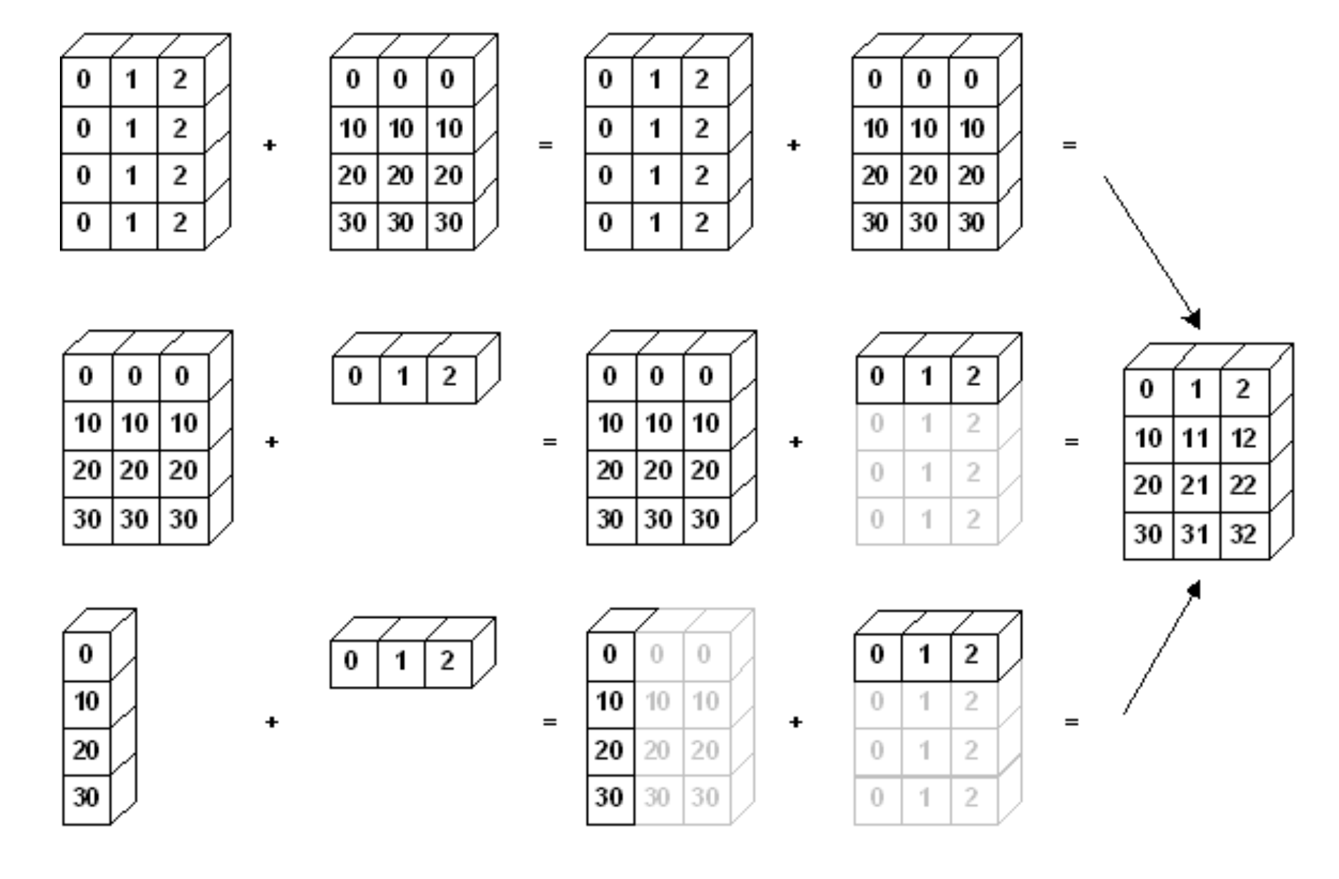
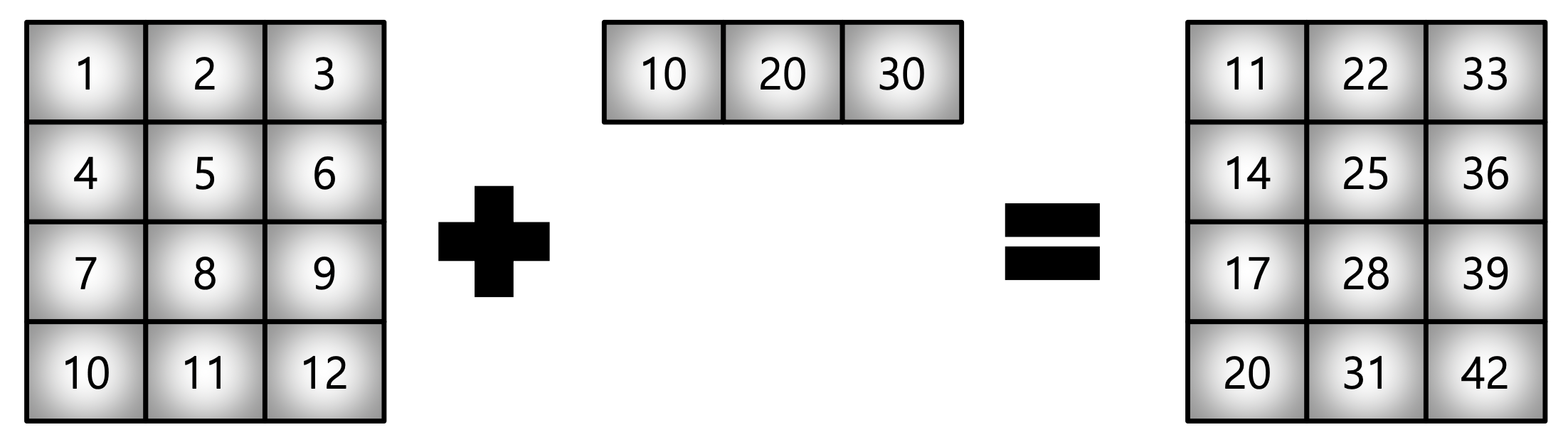
test_matrix = np.arange(1, 13).reshape(4, 3)
test_vector = np.arange(10, 40, 10)
test_matrix + test_vectorarray([[11, 22, 33],
[14, 25, 36],
[17, 28, 39],
[20, 31, 42]])6) Numpy Performance #1
- timeit : Jupyter 환경에서 코드의 Performance를 체크하는 Function
import numpy as np

def scalar_vector_product(scalar, vector):
    result = []
    for value in vector:
        result.append(scalar * value)
    return result

iternation_max = 100000000

vector = list(range(iternation_max))
scalar = 2

%timeit scalar_vector_product(scalar, vector) # for loop을 이용한 성능
%timeit [scalar * value for value in range(iternation_max)] # List Comprehension을 이용한 성능
%timeit np.arange(iternation_max) * scalar # Numpy를 이용한 성능- 일반적으로 속도는
For Loop < List Comprehension < Numpy 순이다. - 100,000,000번의 Loop이 돌 때, 약 4배 이상의 성능 차이를 보임
- Numpy는 C로 구현되어 있어, 성능을 확보하는 대신 Python의 가장 큰 특징인 Dynamic Typing을 포기함
- 대용량 계산에서는 가장 흔히 사용됨
- Concatenate처럼 계산이 아닌, 할당에서는 연산 속도의 이점이 없음
07_Comparisons
1) All & Any
- Array Data 전부(and) 또는 일부(or)가 조건에 만족 여부 Return
a = np.arange(10)
print(a)
np.any(a > 5), np.any(a < 0) # 하나라도 조건에 만족한다면 True
np.all(a > 5), np.all(a < 10) # 모두가 조건에 만족한다면 True[0 1 2 3 4 5 6 7 8 9]
(True, False)
(False, True)2) Comparison Operation #1
- Numpy는 Array의 크기가 동일할 때 Element 간 비교의 결과를 Boolean Type으로 Return
test_a = np.array([1, 3, 0], float)
test_b = np.array([5, 2, 1], float)
test_a > test_b
test_a == test_b
(test_a > test_b).any()array([False, True, False])
array([False, False, False])
Truea = np.array([1, 3, 0], float)
np.logical_and(a > 0, a < 3) # AND 조건의 Condition
b = np.array([True, False, True], bool)
np.logical_not(b) # NOT 조건의 Condition
c = np.array([False, True, False], bool)
np.logical_or(b, c) # OR 조건의 Conditionarray([ True, False, False])
array([False, True, False])
array([ True, True, True])3) Np.where
# np.where(condition, TRUE, FALSE)
np.where(a > 0, 3, 2)

a = np.arange(10) # Index값 Return
np.where(a > 5)

a = np.array([1, np.NaN, np.Inf], float)
np.isnan(a) # Not a Number

np.isfinite(a) # is finite numberarray([3, 3, 2])
(array([6, 7, 8, 9]),)
array([False, True, False])
array([ True, False, False])4) Argmax & Argmin
- Array 안의 최대값 또는 최소값의 Index Return
a = np.array([1, 2, 4, 5, 8, 78, 23, 3])
np.argmax(a), np.argmin(a)
# (5, 0)- Axis 기반의 Return
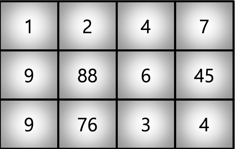
a = np.array([[1, 2, 4, 7], [9, 88, 6, 45], [9, 76, 3, 4]])
np.argmax(a, axis=1), np.argmin(a, axis=0)
# (array([3, 1, 1]), array([0, 0, 2, 2]))
08_Boolean & Fancy Index
1) Boolean Index
- 특정 조건에 따른 값을 Array 형태로 추출
- Comparison Operation Function들도 모두 사용 가능
test_array = np.array([1, 4, 0, 2, 3, 8, 9, 7], float)
test_array > 3

test_array[test_array > 3] # 조건이 True인 Index의 Element만 추출

condition = test_array < 3
test_array[condition]array([False, True, False, False, False, True, True, True])
array([4., 8., 9., 7.])
array([1., 0., 2.])2) Fancy Index
- Numpy는 Array를 Index Value로 사용해서 값 추출
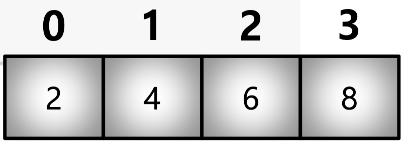
a = np.array([2, 4, 6, 8], float)
b = np.array([0, 0, 1, 3, 2, 1], int) # 반드시 integer로 선언
a[b] # Bracket index, b Array의 값을 Index로 하여 a의 값들을 추출
a.take(b) # take Function : Bracket Index와 같은 효과array([2., 2., 4., 8., 6., 4.])
array([2., 2., 4., 8., 6., 4.])- Matrix 형태의 Data도 가능
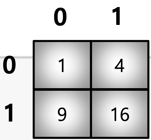
a = np.array([[1, 4], [9, 16]], float)
b = np.array([0, 0, 1, 1, 0], int)
c = np.array([0, 1, 1, 1, 1], int)
a[b, c] # b를 Row Index, c를 Column Index로 변환하여 표시
# array([ 1.,  4., 16., 16.,  4.])
09_Numpy Data I/O
1) Loadtxt & Savetxt
- Text Type의 Data를 읽고, 저장하는 기능
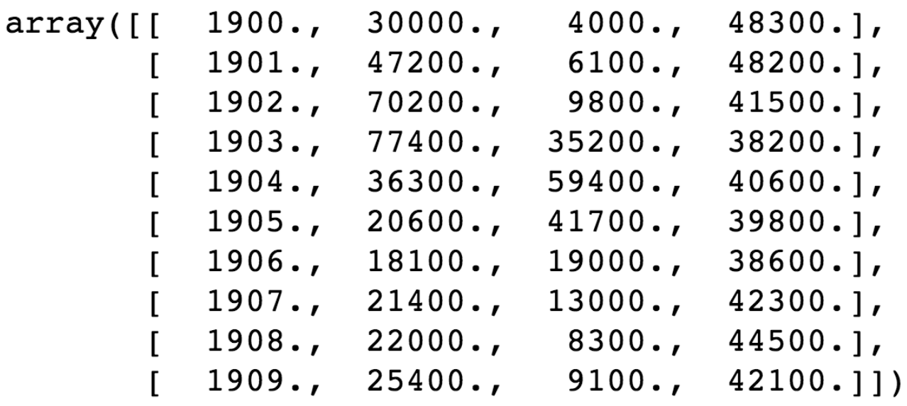
a = np.loadtxt("./populations.txt") # 파일 호출
a[:10]
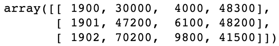
a_int = a.astype(int) # Int Type 변환
a_int[:3]
np.savetxt('int_data.csv', a_int, delimiter=",") # int_data.csv로 저장