새싹 인공지능 응용sw 개발자 양성 교육 프로그램 심선조 강사님 수업 정리 글입니다.
머신러닝을 위한 대표적인 인코딩 방식
- 레이블 인코딩 : 카테고리 피처를 코드형 숫자 값으로 변환하는 것
- 원-핫 인코딩
레이블 인코딩
LableEncoder 클래스로 구현
LableEncoder를 객첼 생성한 후 fit()과 transform()을 호출해 레이블 인코딩을 수행한다.
from sklearn.preprocessing import LabelEncoder
import numpy as np
items = ['TV', '냉장고', '전자레인지', '컴퓨터', '선풍기', '선풍기', '믹서', '믹서']
# 레이블 인코더를 위한 객체 생성
# Encode target labels with value between 0 and n_classes-1.
encoder = LabelEncoder()
# 새로 들어온 데이터는 fit을 하면 안 됨. 기존의 정보가 모두 사라짐.
# 데이터를 사전 작업 하는 것
encoder.fit(items)
# 사전대로 바뀌는 것
# 새로 들어온 데이터는 transform을 해줘야 함
labels = encoder.transform(items)labelsarray([0, 1, 4, 5, 3, 3, 2, 2])encoder.transform(['냉장고'])array([1])# 사전 정보를 확인, 속성값 확인
encoder.classes_array(['TV', '냉장고', '믹서', '선풍기', '전자레인지', '컴퓨터'], dtype='<U5')# 인덱스 값을 원래 값으로 원상복구시키는 것
encoder.inverse_transform([1])array(['냉장고'], dtype='<U5')encoder.inverse_transform(labels)array(['TV', '냉장고', '전자레인지', '컴퓨터', '선풍기', '선풍기', '믹서', '믹서'], dtype='<U5')- 교재 118p
레이블 인코딩을 통해 구분하기 위한 숫자값으로 변환된다. 구분하기 위한 숫자값을 ML알고리즘에서 숫자값을 가중치가 더 부여되거나 더 중요하게 인식할 수 있다. 이러한 특성때문에 선형회귀와 같은 ML알고리즘에는 적용하지 않아야 한다. 트리 계열의 ML알고리즘은 숫자의 이러한 특성을 반영하지 않기에 레이블 인코딩 사용해도 괜찮다. 이러한 문제점을 해결하기 위해서 나온 것이 원-핫 인코딩이다.
분류는 숫자의 크고 작음에 영향을 받지 않음
회귀는 숫자의 크고 작음에 영향을 받음
원-핫 인코딩(one-hot encoding)
피처 값의 유형에 따라 새로운 피처를 추가해 고유 값에 해당하는 칼럼에만 1을 표시하고 나머지 칼럼에는 0을 표시하는 방식이다. 행 행텨로 돼 있는 피처의 교유 값을 열 형태로 차원을 변환한 뒤 고유 값에 해당하는 칼럼에만 1을 표시하고 나머지 칼럼에는 0을 표시한다.
즉, 해당 고유 값에 매칭되는 피처만 1이되고 나머지 피처는 0을 입력하며, 이러한 특성으로 원-핫(여러 개의 속성 중 단 한 개의 속성만 1로 표시)인코딩이라고 한다.
원-핫 인코딩은 사이킷런에서 OneHotEncoder 클래스로 변환이 가능
조건 1. 2차원 데이터 입력값 필요
조건 2. OneHotEncoder를 이용해 반환한 값이 희소 행렬 형태이므로 이를 다시 toarray() 메서드를 이용해 밀집 행렬로 변환해야 한다.
from sklearn.preprocessing import OneHotEncoder
import numpy as np

#numpy
#reshape(-1, 1)에서 -1은 리스트의 총 개수가 몇 개인지 모를 때 -1을 넣음으로써 모양을 뒤의 숫자로 reshape 할 수 있게 만들어줌!
#reshape(4, 2) = reshape(-1, 2)
#reshape(2, 4) = reshape(-1, 4)
# 벡터형태 1차원인데 원핫인코딩을 하기 위해서는 2차원 형태가 필요함
items
# array로 변경 후 reshape해주기, 2차원 ndarry로 변환
items_t = np.array(items).reshape(-1, 1) #reshape(-1, 1) = 리스트안의 원소 개수만큼 행으로 만들어 주기 위함
items_t
# 리스트의 리스트 중첩으로 만들어서 사용
items_l = [['TV'],
['냉장고'],
['전자레인지'],
['컴퓨터'],
['선풍기'],
['선풍기'],
['믹서'],
['믹서']]#원-핫 인코딩 적용
oh_encoder = OneHotEncoder()
oh_encoder.fit(items_l)
result = oh_encoder.transform(items_l)
result.toarray()
# ValueError: Expected 2D array, got 1D array instead : shape이 맞지 않다는 오류array([[1., 0., 0., 0., 0., 0.],
[0., 1., 0., 0., 0., 0.],
[0., 0., 0., 0., 1., 0.],
[0., 0., 0., 0., 0., 1.],
[0., 0., 0., 1., 0., 0.],
[0., 0., 0., 1., 0., 0.],
[0., 0., 1., 0., 0., 0.],
[0., 0., 1., 0., 0., 0.]])oh_encoder = OneHotEncoder()
oh_encoder.fit(items_t)
result = oh_encoder.transform(items_t)
result.toarray() # nd.array로 바꿔서 나타낸array([[1., 0., 0., 0., 0., 0.],
[0., 1., 0., 0., 0., 0.],
[0., 0., 0., 0., 1., 0.],
[0., 0., 0., 0., 0., 1.],
[0., 0., 0., 1., 0., 0.],
[0., 0., 0., 1., 0., 0.],
[0., 0., 1., 0., 0., 0.],
[0., 0., 1., 0., 0., 0.]])oh_encoder.categories_[array(['TV', '냉장고', '믹서', '선풍기', '전자레인지', '컴퓨터'], dtype='<U5')]# 기본 형태가 실수형이라서 숫자 뒤에 점을 찍은거고, 없어도 알아서 실수 형태로 변경됨
oh_encoder.inverse_transform([[1., 0., 0., 0., 0., 0.]])array([['TV']], dtype='<U5')oh_encoder.transform([['냉장고']]).toarray()array([[0., 1., 0., 0., 0., 0.]])get_dummies()
원-핫 인코딩을 더 쉽게 지원하는 api
문자열 카테고리 값을 숫자 형으로 변환할 필요 없이 바로 반환 가능
import pandas as pddf = pd.DataFrame({'item' : ['TV','냉장고','전자레인지','컴퓨터','선풍기']})
df| item | |
|---|---|
| 0 | TV |
| 1 | 냉장고 |
| 2 | 전자레인지 |
| 3 | 컴퓨터 |
| 4 | 선풍기 |
pd.get_dummies(df['item']) #item컬럼을 가지고 만들고 만듦
# pd.get_dummies(df)으로 해도 괜찮음 # 특정컬럼을 지정 안 해서 TV_item으로 나옴| TV | 냉장고 | 선풍기 | 전자레인지 | 컴퓨터 | |
|---|---|---|---|---|---|
| 0 | 1 | 0 | 0 | 0 | 0 |
| 1 | 0 | 1 | 0 | 0 | 0 |
| 2 | 0 | 0 | 0 | 1 | 0 |
| 3 | 0 | 0 | 0 | 0 | 1 |
| 4 | 0 | 0 | 1 | 0 | 0 |
- 교재 122p
피처 스케일링과 정규화
피처 스케일링 : 서로 다른 변수의 값 범위를 일정한 수준으로 맞추는 작업
대표적인 방법으로 표준화(standardization)와 정규화(normalization)가 있다.
표준화
데이터의 피처 각각의 평균이 0이고 분산이 1인 가우시안 정규 분포를 가진 값으로 변환
정규화
서로 다른 피처의 크기를 통일하기 위해 크기를 변환
개별 데이터의 크기를 모두 똑같은 단위로 변경
예시) cm와 \있고 값이 나타내는 범위도 다를 때
같은 잣대로 볼 수 있도록 값의 범위를 같은 값으로 맞추는 것
- 사이킷런에서 제공하는 대표적인 피처 스케일링 클래스: StandardScaler, MinMaxScaler
StandardScaler
개별 피처를 평균이 0이고 분산이 1인 값으로 변환해 준다. 이렇게 가우시안 정규 분포를 가질 수 있도록 데이터를 변환하는 것은 몇몇 알고리즘에서 매우 중요
from sklearn.datasets import load_irisiris = load_iris(as_frame=True) #as_frame=True 데이터프레임으로 가져온다
iris.data.mean() # 평균하고 분산을 구한다sepal length (cm) 5.843333
sepal width (cm) 3.057333
petal length (cm) 3.758000
petal width (cm) 1.199333
dtype: float64iris.data.var() #분산sepal length (cm) 0.685694
sepal width (cm) 0.189979
petal length (cm) 3.116278
petal width (cm) 0.581006
dtype: float64from sklearn.preprocessing import StandardScalerscaler = StandardScaler()
scaler.fit(iris.data)
iris_scaled = scaler.transform(iris.data)iris_df = pd.DataFrame(iris_scaled)iris_df.mean().round(5) # 평균은 0으로 맞춰짐0 -0.0
1 -0.0
2 -0.0
3 -0.0
dtype: float64iris_df.var() # 분산은 1으로 맞춰짐0 1.006711
1 1.006711
2 1.006711
3 1.006711
dtype: float64MinMaxScaler
데이터 값을 0과 1 사이의 범위 값으로 변환한다.(음수 값이 있으면 -1에서 1값으로 변환한다.)
데이터의 분포가 가우시안 분포가 아닐 경우에 MinMaxScaler 사용
# 0~1사이 값을 맞춰주는 것 : MinMaxScaler
from sklearn.preprocessing import MinMaxScaler
scaler = MinMaxScaler()
scaler.fit(iris.data)
iris_scaled = scaler.transform(iris.data)iris_df = pd.DataFrame(iris_scaled)
iris_df.min(),iris.data.min() #값이 0으로 맞춰짐(0 0.0
1 0.0
2 0.0
3 0.0
dtype: float64,
sepal length (cm) 4.3
sepal width (cm) 2.0
petal length (cm) 1.0
petal width (cm) 0.1
dtype: float64)iris_df.max(),iris.data.max() #값이 1으로 맞춰짐(0 1.0
1 1.0
2 1.0
3 1.0
dtype: float64,
sepal length (cm) 7.9
sepal width (cm) 4.4
petal length (cm) 6.9
petal width (cm) 2.5
dtype: float64)가우시안 분포일 때는 스탠다스스케일러 사용
가우시안 정규분포가 아니면 minmax사용
처음에 전체데이터를 fit하고 transform 사용
학습 데이터와 테스트 데이터의 스케일링 변환 시 유의점
StandardScaler이나 MinMaxScaler와 같은 Scaler 객체를 이용해 데이터의 스케일링 변환 시 fit(), transform(), fit_transform() 메서드 사용
fit() - 데이터 변환을 위한 기준 정보 설정
transform() - 설정된 정보를 이용해 데이터 변환
fit_transform() - fit(), transform()을 한 번에 수행
학습데이터로 fit()이 적용된 스케일링 기준 정보를 그대로 테스트 데이터에 적용해야 함. 그렇지 않고 테스트 데이터로 다시 새로운 스케일링 기준 정보를 만들게 되면 학습 데이터와 테스트 데이터의 스케일링 기준 정보가 서로 달라져서 올바른 예측 불가
- 가능하면 전체 데이터의 스케일링 변환 적용 후 학습과 테스트 데이터로 분리
- 1이 여의치 않다면 테스트 데이터 변ㄴ환 시에는 fit()이나 fit_transform()을 적용하지 않고 학습 데이터로 이미 fit()된 Sclar객체를 이용해 transform()으로 변환
# 가우시안 분포
# 가우시안 정규분포가 아니면 minmax 사용
#한 행에 컬럼 하나씩 들어가게끔
train_array = np.arange(0,11).reshape(-1,1)
train_array
array([[ 0],
[ 1],
[ 2],
[ 3],
[ 4],
[ 5],
[ 6],
[ 7],
[ 8],
[ 9],
[10]])test_array = np.arange(0,6).reshape(-1,1)
test_arrayarray([[0],
[1],
[2],
[3],
[4],
[5]])scaler = MinMaxScaler()
scaler.fit(train_array)
train_array = scaler.transform(train_array)# 0~1사이의 값으로 나옴
train_arrayarray([[0. ],
[0.1],
[0.2],
[0.3],
[0.4],
[0.5],
[0.6],
[0.7],
[0.8],
[0.9],
[1. ]])# fit을 하고 transform을 하면 0.5가 안 나옴
# 뒤에 추가되는 데이터는 transform만 해줘야 함
# scaler.fit(test_array)
scaler.fit(test_array)
test_array = scaler.transform(test_array)test_arrayarray([[0. ],
[0.2],
[0.4],
[0.6],
[0.8],
[1. ]])#fit을 안 했을 때 결과
#scaler.fit(test_array)
test_array = scaler.transform(test_array)test_arrayarray([[0. ],
[0.04],
[0.08],
[0.12],
[0.16],
[0.2 ]])- 교재 130p
캐글에서 제공하는 타이타닉 생존자 예측(titanic.csv)
https://www.kaggle.com/competitions/titanic
import pandas as pd
import numpy as np
import matplotlib.pyplot as plt
import seaborn as sns
df = pd.read_csv('titanic.csv')
df.head(2)| PassengerId | Survived | Pclass | Name | Sex | Age | SibSp | Parch | Ticket | Fare | Cabin | Embarked | |
|---|---|---|---|---|---|---|---|---|---|---|---|---|
| 0 | 1 | 0 | 3 | Braund, Mr. Owen Harris | male | 22.0 | 1 | 0 | A/5 21171 | 7.2500 | NaN | S |
| 1 | 2 | 1 | 1 | Cumings, Mrs. John Bradley (Florence Briggs Th... | female | 38.0 | 1 | 0 | PC 17599 | 71.2833 | C85 | C |
df.info()<class 'pandas.core.frame.DataFrame'>
RangeIndex: 891 entries, 0 to 890
Data columns (total 12 columns):
# Column Non-Null Count Dtype
--- ------ -------------- -----
0 PassengerId 891 non-null int64
1 Survived 891 non-null int64
2 Pclass 891 non-null int64
3 Name 891 non-null object
4 Sex 891 non-null object
5 Age 714 non-null float64
6 SibSp 891 non-null int64
7 Parch 891 non-null int64
8 Ticket 891 non-null object
9 Fare 891 non-null float64
10 Cabin 204 non-null object
11 Embarked 889 non-null object
dtypes: float64(2), int64(5), object(5)
memory usage: 83.7+ KB#비어있는 데이터는 메꾸던가 비우던가
#나이는 평균값으로 또는 객실은 n(=없음)으로 메꿔놓는다 ex)10 Cabin 204 non-null object
df.isnull().sum()PassengerId 0
Survived 0
Pclass 0
Name 0
Sex 0
Age 177
SibSp 0
Parch 0
Ticket 0
Fare 0
Cabin 687
Embarked 2
dtype: int64df['Age'].fillna(df['Age'].mean(),inplace=True)
df['Cabin'].fillna('N',inplace=True)
df['Embarked'].fillna('N',inplace=True)df.isnull().sum()PassengerId 0
Survived 0
Pclass 0
Name 0
Sex 0
Age 0
SibSp 0
Parch 0
Ticket 0
Fare 0
Cabin 0
Embarked 0
dtype: int64df.info()<class 'pandas.core.frame.DataFrame'>
RangeIndex: 891 entries, 0 to 890
Data columns (total 12 columns):
# Column Non-Null Count Dtype
--- ------ -------------- -----
0 PassengerId 891 non-null int64
1 Survived 891 non-null int64
2 Pclass 891 non-null int64
3 Name 891 non-null object
4 Sex 891 non-null object
5 Age 891 non-null float64
6 SibSp 891 non-null int64
7 Parch 891 non-null int64
8 Ticket 891 non-null object
9 Fare 891 non-null float64
10 Cabin 891 non-null object
11 Embarked 891 non-null object
dtypes: float64(2), int64(5), object(5)
memory usage: 83.7+ KBdf['Sex'].value_counts() #value_counts()를 하면 유일값을 꺼내서 개수를 세어준다male 577
female 314
Name: Sex, dtype: int64df['Cabin'].value_counts()N 687
C23 C25 C27 4
G6 4
B96 B98 4
C22 C26 3
...
E34 1
C7 1
C54 1
E36 1
C148 1
Name: Cabin, Length: 148, dtype: int64df['Embarked'].value_counts()S 644
C 168
Q 77
N 2
Name: Embarked, dtype: int64#첫 글자 추출 str
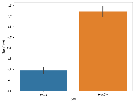
df['Cabin'] = df['Cabin'].str[:1]df.groupby(['Sex','Survived'])['Survived'].count() #그룹으로 묶어서 행의 개수세기Sex Survived
female 0 81
1 233
male 0 468
1 109
Name: Survived, dtype: int64sns.barplot(data=df,x='Sex',y='Survived')<AxesSubplot:xlabel='Sex', ylabel='Survived'>
sns.barplot(data=df,x='Pclass',y='Survived',hue='Sex')<AxesSubplot:xlabel='Pclass', ylabel='Survived'>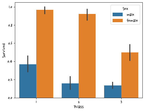
df['Age'].value_counts() 29.699118 177
24.000000 30
22.000000 27
18.000000 26
28.000000 25
...
36.500000 1
55.500000 1
0.920000 1
23.500000 1
74.000000 1
Name: Age, Length: 89, dtype: int64def get_category(age):
cat=''
if age <= -1: cat='Unknown'
elif age <= 5: cat = 'Baby'
elif age <= 12: cat = 'Child'
elif age <= 18: cat = 'Teenager'
elif age <= 25: cat = 'Student'
elif age <= 35: cat = 'Young Adult'
elif age <= 60: cat = 'Adult'
else : cat = 'Elderly'
return catdf['Age_cat'] = df['Age'].apply(lambda x : get_category(x))plt.figure(figsize=(10,6)) #사이즈 설정
group_name = ['Unknown','Baby','Child','Teenager','Student','Young Adult','Adult','Elderly']
sns.barplot(data=df,x='Age_cat',y='Survived',hue='Sex', order=group_name)<AxesSubplot:xlabel='Age_cat', ylabel='Survived'>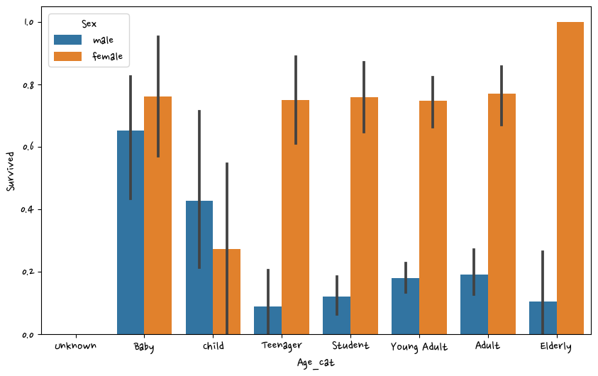
문자열 피처는 인식을 못 하서 숫자형으로 바꿔줘야 한다. -> labelEncoder사용
회귀쪽 모델은 숫자에 따라서 영향을 미친다. 분류쪽 모델은 숫자에 영향을 거의 안 받아서 labelEncoder사용
from sklearn.preprocessing import LabelEncoder #함수를 만들어서 데이터 fit 처리하도록 만듦
def encode_features(dataDF):
features=['Sex','Cabin','Embarked']
for feature in features:
le = LabelEncoder()
dataDF[feature] = le.fit_transform(dataDF[feature])
print(le.classes_)#레이블인코더 확인 할 때 = class
return dataDFdf = encode_features(df)
df.head(2) #문자형을 숫자형으로 바꿈['female' 'male']
['A' 'B' 'C' 'D' 'E' 'F' 'G' 'N' 'T']
['C' 'N' 'Q' 'S']| PassengerId | Survived | Pclass | Name | Sex | Age | SibSp | Parch | Ticket | Fare | Cabin | Embarked | Age_cat | |
|---|---|---|---|---|---|---|---|---|---|---|---|---|---|
| 0 | 1 | 0 | 3 | Braund, Mr. Owen Harris | 1 | 22.0 | 1 | 0 | A/5 21171 | 7.2500 | 7 | 3 | Student |
| 1 | 2 | 1 | 1 | Cumings, Mrs. John Bradley (Florence Briggs Th... | 0 | 38.0 | 1 | 0 | PC 17599 | 71.2833 | 2 | 0 | Adult |
def fillna(df):
df['Age'].fillna(df['Age'].mean(),inplace=True)
df['Cabin'].fillna('N',inplace=True)
df['Embarked'].fillna('N',inplace=True)
df['Fare'].fillna(0, inplace=True)
return df
def drop_features(df):
df.drop(columns=['PassengerId', 'Name', 'Ticket'], inplace=True)
return df
def format_features(df):
from sklearn.preprocessing import LabelEncoder #함수안에 같이 넣어주는 것이 좋음
df['Cabin'] = df['Cabin'].str[:1] #Cabin의 첫 번째 글자만 추출
features=['Sex','Cabin','Embarked']
for feature in features:
le = LabelEncoder()
df[feature] = le.fit_transform(df[feature])
print(le.classes_) #레이블인코더 확인 할 때 = class
return df
def transform_features(df): #함수 3개 호출
df = fillna(df)
df = drop_features(df)
df = format_features(df)
return df
df = pd.read_csv('titanic.csv')
#df = pd.read_csv('titanic.csv')
y = df['Survived']
X = df.drop(columns=['Survived'])
#X = transform_features(X)X = transform_features(X)['female' 'male']
['A' 'B' 'C' 'D' 'E' 'F' 'G' 'N' 'T']
['C' 'N' 'Q' 'S']X.head(2)| Pclass | Sex | Age | SibSp | Parch | Fare | Cabin | Embarked | |
|---|---|---|---|---|---|---|---|---|
| 0 | 3 | 1 | 22.0 | 1 | 0 | 7.2500 | 7 | 3 |
| 1 | 1 | 0 | 38.0 | 1 | 0 | 71.2833 | 2 | 0 |
from sklearn.model_selection import train_test_splitX_train,X_test,y_train,y_test = train_test_split(X,y,test_size=0.2,random_state=11)from sklearn.tree import DecisionTreeClassifier
from sklearn.ensemble import RandomForestClassifier
from sklearn.linear_model import LogisticRegression
from sklearn.metrics import accuracy_scoredt_clf = DecisionTreeClassifier(random_state=11)
rf_clf = RandomForestClassifier(random_state=11)
lr_clf = LogisticRegression(solver='liblinear') dt_clf.fit(X_train,y_train)
dt_pred = dt_clf.predict(X_test)
accuracy_score(y_test,dt_pred)0.7877094972067039rf_clf.fit(X_train,y_train)
rf_pred = rf_clf.predict(X_test)
accuracy_score(y_test,rf_pred)0.8547486033519553#LogisticRegression
lr_clf.fit(X_train,y_train)
lr_pred = lr_clf.predict(X_test)
accuracy_score(y_test,lr_pred)0.8659217877094972from sklearn.model_selection import GridSearchCVparam = {
'max_depth':[2, 3, 5, 10], #3이라면 몇 번 내려갈 것이냐
'min_samples_split':[2, 3, 4], # 3이라면 최소 3이 있어야 가지치기를 할 수 있다
'min_samples_leaf':[1, 5, 8]} # 가장 마지막grid = GridSearchCV(dt_clf, param, cv=5, scoring='accuracy')
grid.fit(X_train,y_train)GridSearchCV(cv=5, estimator=DecisionTreeClassifier(random_state=11),
param_grid={'max_depth': [2, 3, 5, 10],
'min_samples_leaf': [1, 5, 8],
'min_samples_split': [2, 3, 4]},
scoring='accuracy')pred = grid.predict(X_test)accuracy_score(y_test,pred)0.8715083798882681grid.best_params_{'max_depth': 3, 'min_samples_leaf': 5, 'min_samples_split': 2}평가
머신러닝은 데이터 가공/변환, 모델 학습/예측, 평가의 프로세스로 구성
타이타닉 생존자 예제에서 모델 예측 성능의 평가를 위해 정확도를 이용
성능 평가 지표(Evaluation Metric)는 일반적으로 모델이 분류나 회귀에 따라 여러 종류로 나뉜다.
회귀와 분류의 평가는 다르다.
-
회귀
회귀는 결과값이 연속값으로 나온다. 연속값으로 나오기 때문에 적중해서(똑같이) 맞출 수 없다. 그래서 차이가 작게 나면 좋은 것이다. 회귀는 w,b값을 찾는 과정이다. 나온 오차를 보고 미분을 해서 +-보고 w를 더하고 빼준다. -
분류
정확도만으로 평가가 안 되는 데이터가 있다. 이진분류는 0아니면 1로 구성되어 정확도보다는 다른 성능 평가 지표가 더 중요시 됨
분류의 성능 평가 지표 : 정확도, 오차행렬, 정밀도, 재현율, f1스코어, ROC AUC
정확도 = 예측 결과가 동일한 데이터 건수 / 전체 예측 데이터 건수
#모델만들기
from sklearn.base import BaseEstimator
from sklearn.model_selection import train_test_split
import pandas as pd
from sklearn.metrics import accuracy_score
import numpy as np
class MyDummyClassifier(BaseEstimator): #클래스이름 옆에 ()하면 상속이다. BaseEstimator을 상속받겠다
def fit(self, X, y=None): #fit()메서드는 아무것도 학습하지 않음, pass =함수안에 아무 것도 정의 안 하고 넘어간다
pass
def predict(self, X):
pred = np.zeros((X.shape[0], 1)) #행은 데이터의 건수다. column = 레이블값 1
for i in range(X.shape[0]): #데이터 건수(행)을 가져다가
if X['Sex'].iloc[i] == 1: #성별이 1=남자라면
pred[i] = 0 #결과값에 0을 넣어줘라
else:
pred[i] = 1
return pred파이썬에서 클래스를 만들 때 class를 만들고 단어의 첫 글자는 대문자
다중상속 가능
첫 번째 파라미터값은 self으로 보통 적는다. 내부적으로 주소값을 받는다. self는 없는 것이다.
두 번째 파라미터값은 내가 맘대로 정의해도 괸다.
def fillna(df):
    df['Age'].fillna(df['Age'].mean(),inplace=True)
    df['Cabin'].fillna('N',inplace=True)
    df['Embarked'].fillna('N',inplace=True)
    df['Fare'].fillna(0, inplace=True)
    return df

def drop_features(df):
    df.drop(columns=['PassengerId', 'Name', 'Ticket'], inplace=True)
    return df

def format_features(df):
    from sklearn.preprocessing import LabelEncoder  #함수안에 같이 넣어주는 것이 좋음
    df['Cabin'] = df['Cabin'].str[:1] #Cabin의 첫 번째 글자만 추출
    features=['Sex','Cabin','Embarked']
    for feature in features:
        le = LabelEncoder()
        df[feature] = le.fit_transform(df[feature])
        print(le.classes_) #레이블인코더 확인 할 때 = class
    return df

def transform_features(df): #함수 3개 호출
    df = fillna(df)
    df = drop_features(df)
    df = format_features(df)
    return df

df = pd.read_csv('titanic.csv')
y = df['Survived']
X = df.drop(columns=['Survived'])
X = transform_features(X)
X_train,X_test,y_train,y_test = train_test_split(X,y,test_size=0.2,random_state=11)
['female' 'male']
['A' 'B' 'C' 'D' 'E' 'F' 'G' 'N' 'T']
['C' 'N' 'Q' 'S']myclf = MyDummyClassifier()
myclf.fit(X_train,y_train)
pred = myclf.predict(X_test)
accuracy_score(y_test,pred)
0.8324022346368715이진분류로 바꾸려면 2가지 경우만 있어야 한다.
true, false면 bool형태다.
astype(int)하면
true -> 1 , false -> 2으로 된다.
이진분류에서 데이터의 불균형이 심할 때 단순히 정확도만 가지고 평가하면 문제가 있다.
이것을 해결하기 위해서 오차행렬을 사용한다.
오차행렬
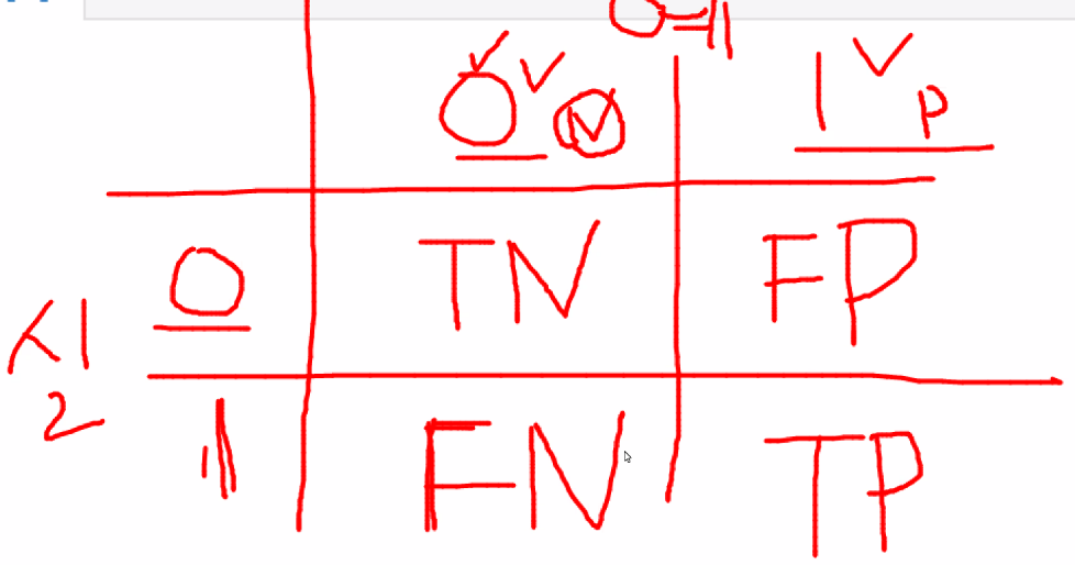
from sklearn.metrics import confusion_matrixconfusion_matrix(y_test,pred) #이 숫치값을 통해서 평가한다array([[103, 15],
[ 15, 46]], dtype=int64)정밀도와 재현율
- 교재 154P
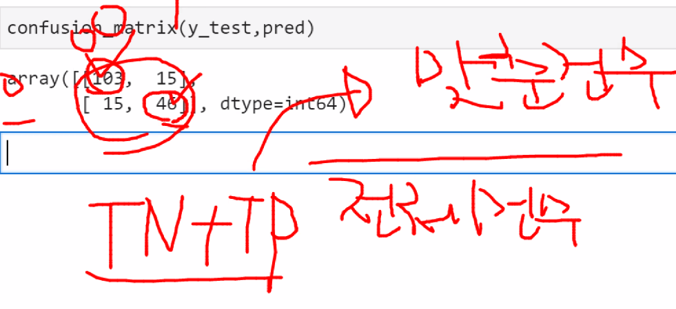
정확도 = 맞춘 건수(TN+TP = 103+46)/ 전체건수(104+15+15+46)
- 교재 153P
내가 1이라고 예측한 값(FP+TP)정밀도 = 내가 1이라고 예측한 값중에서 얼마나 맞췄느냐 = TP/TP+FP
(기준 :내가 예측한 값)
재현율 = 실제값(1)을 기준으로 얼마나 맞췄느냐 = TP / FN+TP
(기준: 실제 값)
보통 정밀도와 재현율은 같이 안 간다. 정밀도가 올라가면 재현율은 떨어진다.
정밀도와 재현율은 상황에 따라서 중요하게 보는 것이 다르다.
-교재 155P
재현율이 상대적으로 더 중요한 지표인 경우는 실제 Positive 양성인 데이터 예측을 Negative로 잘못 판단하게 되면 업무상 큰 영향이 발생하는 경우
정밀도가 상대적으로 더 중요한 지표인 경우는 실제 Negative 음성인 데이터 예측을 Positive 양성으로 잘못 판단하게 되면 업무상 큰 영향이 발생하는 경우
평가 - 이 모델이 진짜 사용할 수 있는 것이냐
이진분류 한 쪽으로 쏠려있을 경우 정확도가 높을 수 있다.
그래서 이것 말고 다른 정확도를 판단할 수 있는 방법이 있다.