새싹 인공지능 응용sw 개발자 양성 교육 프로그램 심선조 강사님 수업 정리 글입니다.

머신러닝
컴퓨터 스스로! 학습! -> 머신러닝
머신러닝 안의 한 형태 -> 딥러닝
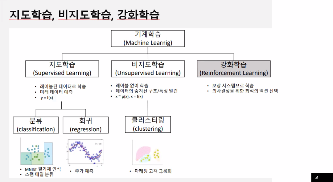

머신러닝 - 지도 학습, 비지도 학습, 강화 학습
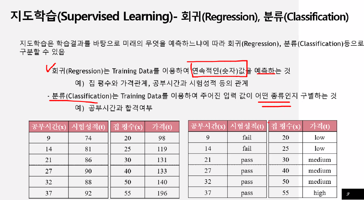
지도학습
레이블 = 정답
답을 주고 학습 -> 지도학습 -> 예측
- 분류 -> 이상값에 대한 결과
- 회귀 -> 결과값이 연속값으로 나오는 것
회귀를 이해하면 딥러닝을 이해하는 데 편하다.

예시1 = 분류
예시2 = 회귀, 가격(=연속데이터)
왼쪽 = 회귀
오른쪽 = 분류
비지도 학습
레이블 없이 학습
데이터 상태를 보고 끼리끼리묶어줌
- 클러스터링 : 몇 개로 나눌 지 알려줘야 한다.
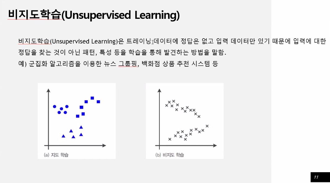
정답을 찾는 것이 아닌 패턴, 특성 등을 학습을 통해 발견
지도학습 - 선형회귀
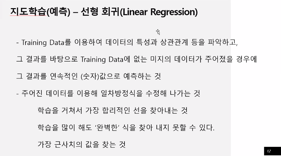
학습하는 데이터를 이용해서 데이터의 특성과 상관관계를 파악
그 결과를 연속적인 숫자값으로 예측하는 것
입력값과 출력값사이에 연관관계가 있어서 결과가 나올 수 있다.
입력값에 아무런 영향을 받지 않으면 결과가 나올 수 없다.
상관계수 -1 ~ 1
1에 가까우면 하나의 값이 증가하면 하나의 값은 감소한다.↑↓
0에 가까우면 관계성이 없다.
1에 가까우면 하나의 값이 증가하면 하나의 값도 증가한다.↑↑
상관관계는 그 쪽에 가까운 쪽으로 데이터를 넣어서 처리하는 것이 좋다. 결과값이 예측할 수 있다. 데이터는 아무거나 선택하는 것이 아니라 관계가 있는 데이터를 골라야 한다.
입력값(=독립변수), 출력값(=종속변수)
독립변수에 영향을 받는 종속변수
주어진 데이터들을 일차방정식으로 나타낼 수 있다.
데이터들 사이에 관계를 일차방정식으로 만들어 볼 수 있다.
일차방정식은 학습을 통해 가장 합리적인 선을 찾아내는 것 = 선형회귀의 목적(가장 근사치의 값을 찾는 것)
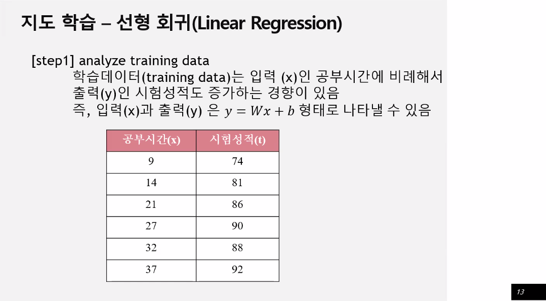
y =wx + b
입력값(x), 결과값(y)는 우리가 안다.머신러닝이 스스로 찾아야 하는 값은 w(가중치, 회귀계수),b(절편)를 찾아야 한다.
일차방정식을 구하기 위한 선형회귀의 목적이다.
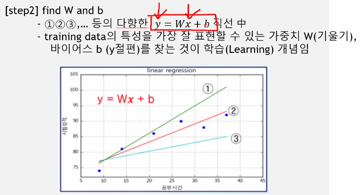
1,2,3(선)과 실제 데이터(점)들에 선을 그읏 것이 오차라고 한다.
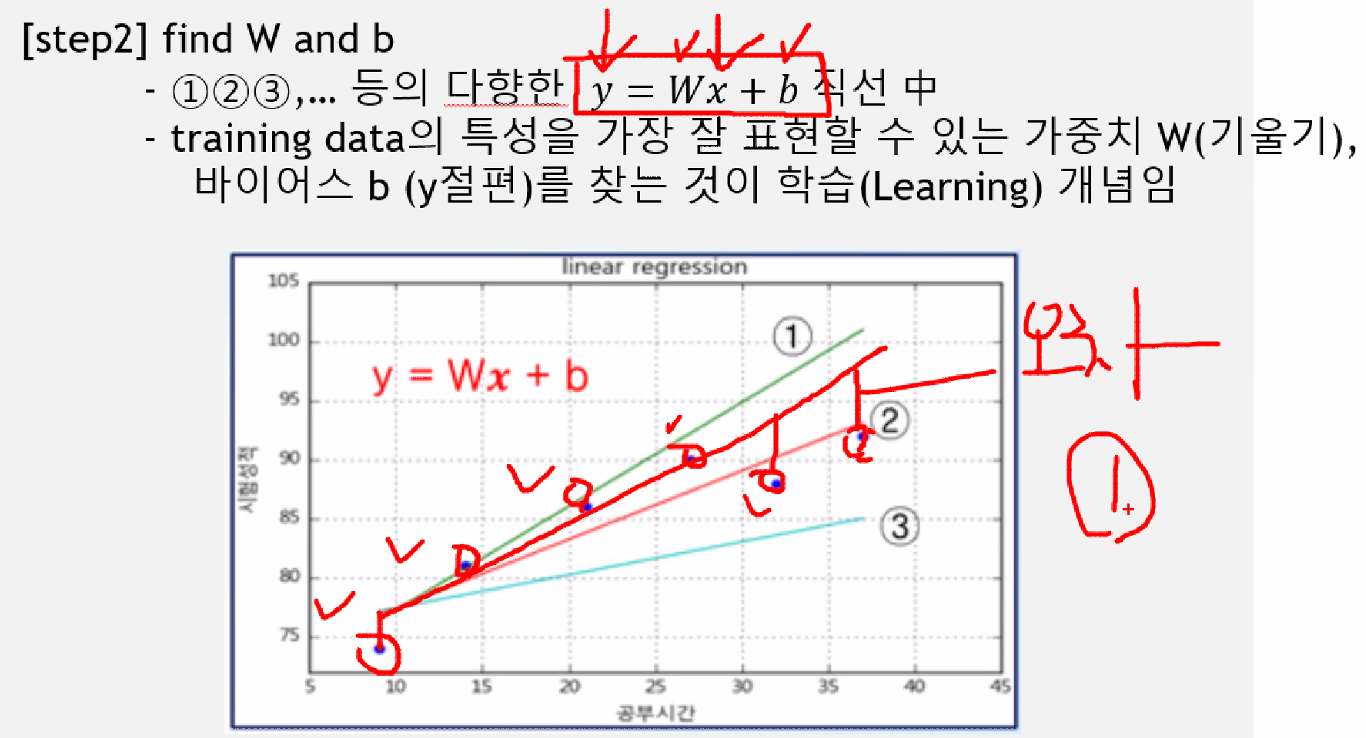

수치값을 하나로 합치려고 할 때 오차의 평균을 낸다. 오차는 +- 값이 있어서 0으로 수렴될 수 있다. -없애기 위해서 절대값 혹은 제곱을 한다. 그 값들의 평균을 내면 대표값으로 처리할 수 있다.
- 선형회귀 요약
직선은 예측하는 값
점은 실제 값
직선과 점을 이은 것 오차
대표값을 구할 때 평균으로 구한다.
오차는 대표값 하나(오차들의 평균)
하지만 오차는 +- 값들이 있어서 0으로 수렴하기 때문에 - 없애기 위해서 절대값또는 제곱을 해준다.
절대값또는 제곱을 둘 중 아무거나 사용해도 되지만
제곱을 좀 더 사용하는 이유는 미분, 적분을 사용할 때 또는 제곱하면 차이값에 예민하게 반응하기 때문이다.
오차값이작으면 좋은 것이다.
여러번에 걸쳐서 오차를 구하는데 첫 시도를 통해 두 번째 시도에는 w,b값이 오차값을 줄이는 방향으로 설정해야 한다.(=경사하강법)
- 일차방정식에 대한 직선을 구한다(직선 = 예측)
- 예측과 실제값에 그은 선을 오차라고 한다.
- w,b를 오차가 줄어드는 방향으로 수정한다.
첫째 시도와 두 번째 시도와 사이에 더 좋은 방향으로 가고 있다는 확신있어야 한다. w,b는 임의의 값이 아닌 오차를 줄어드는 방향으로 수정해야 한다.

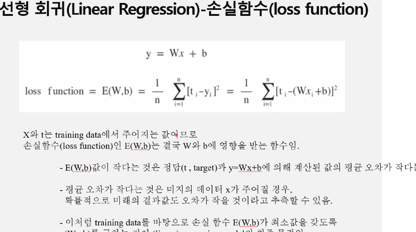
손실함수
경사하강법
- 우리의 목적은 오차가 최소화가 되는 w,b값을 찾는 것
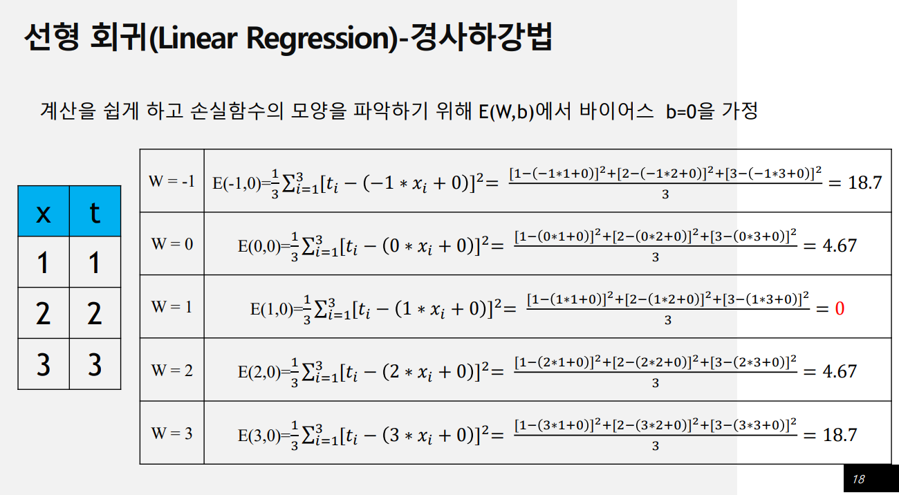
- 손실 함수 E(W,b)를 구하는 것이 (linear) regression model의 최종 목적 -> 경사하강법(gradient decent algorithm)

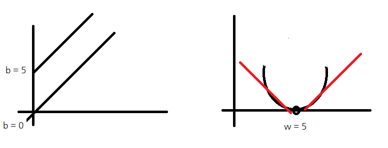
b(절편- 축과 만나는 점)는 보통 임의로 0으로 두고 w에서만 계산한다.
어느 지점에 w값이 되면 오차는 제일 낮은 지점에 있을 것이다.
w중심으로 봤을 때 w=5일 때 오차가 제일 낮다.
오차는 제일 낮은 지점이 있을 거고 제일 낮은 지점을 늘어나면 오차는 늘어난다. 제곱을 사용하면 점점 갈수록 급격하게 늘어난다. 절대값을 사용하면 직선으로 나온다.
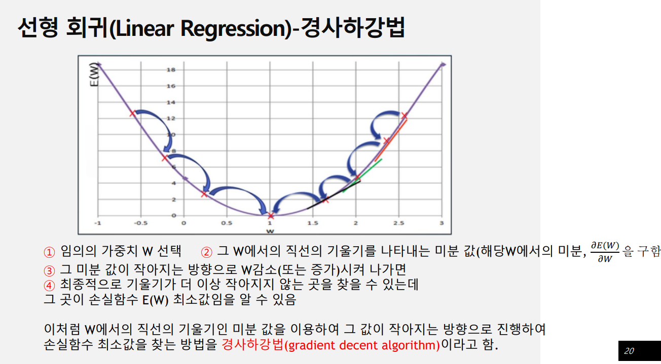

미분을 통해서 기울기를 계산한다.
w값을 더해주면 기울기는 완만한 쪽으로 움직일 것이다.
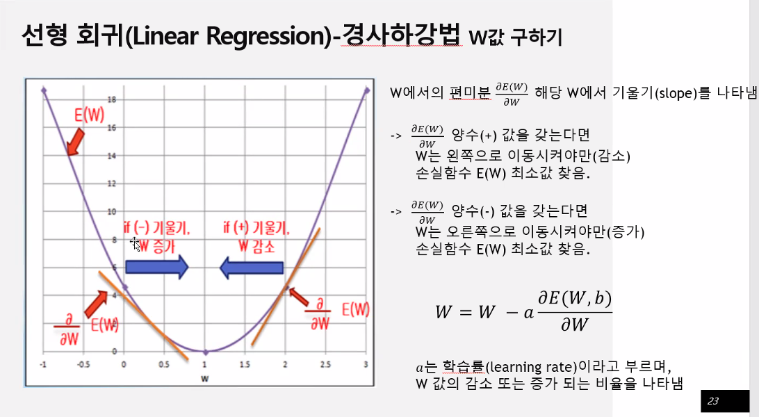
w값을 임의로 정하고 미분을 통해 기울기를 구한다. 기울기가 +값이면 w값을 빼준다. 기울기가 -값이면 w값을 더해준다.
여기서 중요한 것은 w값을 얼마나 더하고 뺄 것이냐
너무 많이 움직이면 바깥으로 튄다.
w를 얼마만큼 움직일 것이냐 = 학습률
조금씩 움직여 가면서 학습을 한다. 적절하게 우리가 움직이면서 학습을 한다. 기울기가 0이 되는 지점으로 가고자 하는 것이다.
지도학습(분류) - 의사결정 트리
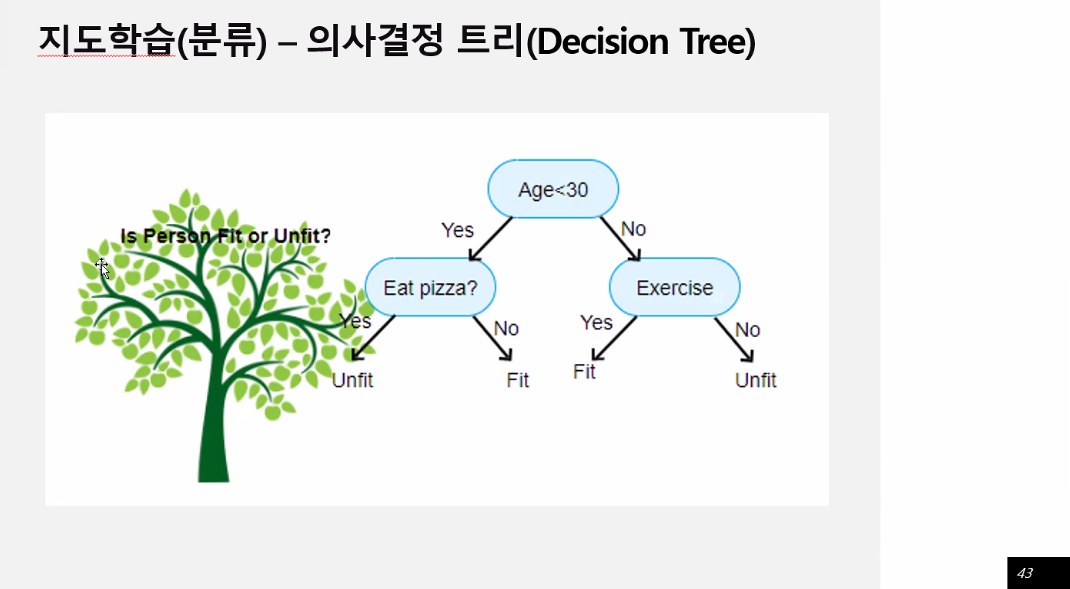
시각화에도 좋다. 간단한데 성능이 나쁘지 않다. 앙상블과 묶어서 사용하면 괜찮은 성능이 있다.
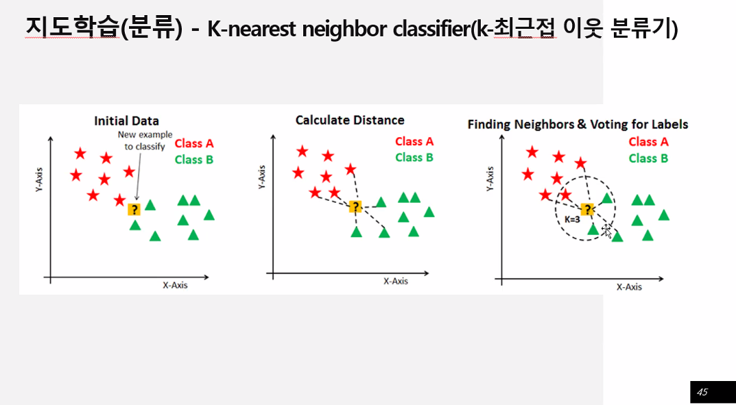
지도학습(분류) - k-최근접 이웃분류기

비지도학습(군집) - 평균 군집
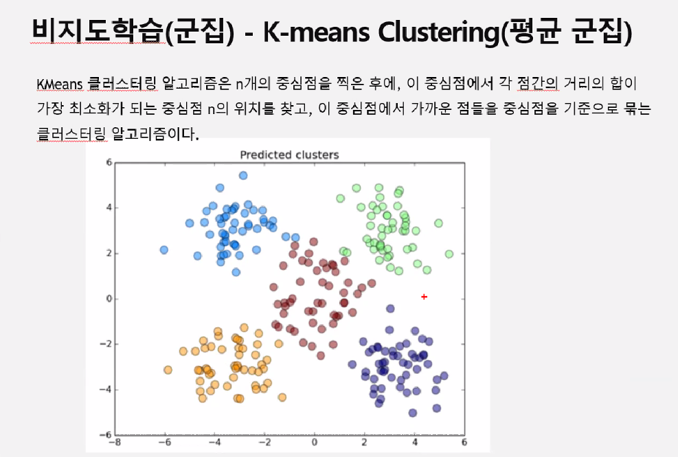
점을 찍는 방법은
중심점에서 각 점간의 거리의 합이 가장 최소화가 되는 중심점 n의 위치를 찾고, 이 중심점에서 가까운 점들을 중심점을 기준으로 묶는 클러스터링 알고리즘이다. 중심점을 안 움직여도 될 때 그만둔다.
강화학습
경쟁으로 통해 더 좋은 결과 도출
- 교재 85p
머신러닝에 사이킷런을 많이 사용한다.
자바(객체지향프로그램) method overriding : 부모로 부터 받은 매소드를 재정의해서 사용
자바 method overoading : class안에 파라미터를 다르게 사용
파이썬에서도 class가 있어서 상속이 가능하다.
학습시키면 fit, 예측은 predict
학습된 것을 fit에 저장, 예측은 predict에 저장
import
0, 0, 0, 0, 0, 0, 0, 0, 0, 0, 0, 0, 0, 0, 0, 0, 0, 0, 0, 0, 0, 0,
0, 0, 0, 0, 0, 0, 1, 1, 1, 1, 1, 1, 1, 1, 1, 1, 1, 1, 1, 1, 1, 1,
1, 1, 1, 1, 1, 1, 1, 1, 1, 1, 1, 1, 1, 1, 1, 1, 1, 1, 1, 1, 1, 1,
1, 1, 1, 1, 1, 1, 1, 1, 1, 1, 1, 1, 2, 2, 2, 2, 2, 2, 2, 2, 2, 2,
2, 2, 2, 2, 2, 2, 2, 2, 2, 2, 2, 2, 2, 2, 2, 2, 2, 2, 2, 2, 2, 2,
2, 2, 2, 2, 2, 2, 2, 2, 2, 2, 2, 2, 2, 2, 2, 2, 2, 2]),
'frame': None,
'target_names': array(['setosa', 'versicolor', 'virginica'],
0 = setosa
1 = versicolor
2 = virginica
-
교재 91p
estimator 이해 및 fit(), predict()메서드 -
교재 98p
model selecting 모듈 소개
데이터를 학습과 평가에 쓸 데이터를 분리한다.
!python -VPython 3.9.13페이지 10p 2문단 - microsoft visual studio build tools 다운
https://visualstudio.microsoft.com/ko/downloads/
import sklearn
sklearn.__version__'1.0.2'피쳐 = 변수 = 입력값= x = 독립변수
- 붓꽃 데이터 피처
sepal length
sepal width
petal length
petal width
from sklearn.datasets import load_iris #제공되는 데이터
from sklearn.tree  import DecisionTreeClassifier #의사결정 트리
#  import DecisionTreeClassifier - 의사결정트리에서 분류에서 사용 DecisionTreeRegressor - 의사결정트리에서 회귀에서 사용
from sklearn.model_selection import train_test_split # 학습, 검증에서 사용할 데이터를 분류한다. train_test_split-데이터를 분리하는 데 사용한다.
#모르는 새로운 데이터를 맞추는 것이 중요하다. 학습한 데이터를 검증하면 정확도 100% 나온다.

import pandas as pd
#import를 먼저 해야 자동완성을 사용할 수 있다. import를 먼저 하는 것이 좋다.
iris = load_iris(as_frame = True) #Dimensionality 4 : 변수 4개 = 4차원
#Features real, positive : freatures = 변수값? - 실수
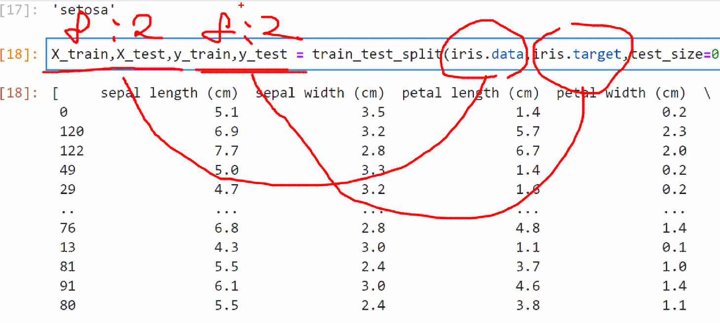
#data = x, target = y
#형태는 딕셔너리같아 보이지만 딕셔너리는 아니다.
#as_frame = True : 데이터 프레임으로 반환한다.iris.data.head(2) #딕셔너리라서 key값으로 접근| sepal length (cm) | sepal width (cm) | petal length (cm) | petal width (cm) | |
|---|---|---|---|---|
| 0 | 5.1 | 3.5 | 1.4 | 0.2 |
| 1 | 4.9 | 3.0 | 1.4 | 0.2 |
iris.target #series형태로 되어 있다.0 0
1 0
2 0
3 0
4 0
..
145 2
146 2
147 2
148 2
149 2
Name: target, Length: 150, dtype: int32iris_df = iris.data
#iris_df['label'] = iris.target #label column 만들어줌
iris_df.head(2)| sepal length (cm) | sepal width (cm) | petal length (cm) | petal width (cm) | |
|---|---|---|---|---|
| 0 | 5.1 | 3.5 | 1.4 | 0.2 |
| 1 | 4.9 | 3.0 | 1.4 | 0.2 |
iris.target_names[0] #0 해당하는 값을 리턴받아라?'setosa'#분리
X_train,X_test,y_train,y_test = train_test_split(iris.data,iris.target,test_size=0.2, random_state=11) #test_size=None, train_size=None 2개 합쳐서 100% #random_state=None 똑같이 나누고 싶으면 고정시킬 수 있다. shuffle = 데이터를 섞어서 나눈다.
#x = iris.data, y = iris.target, test_size=0.2 : 8:2로 나누겠다
#분리된 데이터를 학습할 모델
dt_clf = DecisionTreeClassifier(random_state=11)
#fit할때는 정답도 같이 넣어줘야 한다
dt_clf.fit(X_train,y_train)DecisionTreeClassifier(random_state=11)#예측
pred = dt_clf.predict(X_test) #예측값(pred)과 결과값(y_test) 비교
list(zip(pred, y_test)) [(2, 2),
(2, 2),
(1, 2),
(1, 1),
(2, 2),
(0, 0),
(1, 1),
(0, 0),
(0, 0),
(1, 1),
(1, 2),
(1, 1),
(1, 1),
(2, 2),
(2, 2),
(0, 0),
(2, 2),
(1, 1),
(2, 2),
(2, 2),
(1, 1),
(0, 0),
(0, 0),
(1, 1),
(0, 0),
(0, 0),
(2, 2),
(1, 1),
(0, 0),
(1, 1)]#하나하나 눈으로 맞춰보기 어려우니까
from sklearn.metrics import accuracy_score #평가관련된 것은 모두 metrics안에 있따, import accuacy_score 은 얼마나 정확했는지 비율로 나타남accuracy_score(y_test,pred) #1.0 = 100%(다 맞춤)0.9333333333333333- 빠진 것
- 크롤링
- 전처리
2-1. 전처리할 때도 이렇게 저렇게 할 때 데이터마다 전처리 해줘야 한다.
머신러닝은 숫자로만 처리한다, 글자는 전부다 숫자형태로 바꿔서 들어간다.
숫자형으로 만들고 보기 좋게는 따로 만들어야 한다.
dt_clf.predict([[4.67,3.9,2,0.4]])#데이터를 한 건만 넣은 것이 아니기 때문에 2차원 데이터로 넣어야 한다. -> reshapeC:\anaconda\lib\site-packages\sklearn\base.py:450: UserWarning: X does not have valid feature names, but DecisionTreeClassifier was fitted with feature names
warnings.warn(
array([0])import picklef = open('model', 'wb') #model이라고 저장하고 w = 쓰기모드
pickle.dump(dt_clf,f) #dump 파일로 저장할 때 #f파일로 저장f.close() #model이라는 파일생성f = open('model', 'rb')
model = pickle.load(f) #파일 읽기
f.close()model.predict([[4.67,3.9,2,0.4]])C:\anaconda\lib\site-packages\sklearn\base.py:450: UserWarning: X does not have valid feature names, but DecisionTreeClassifier was fitted with feature names
warnings.warn(
array([0])iris = load_iris() #df기본
type(iris) #sklearn.utils.Bunch - 딕셔너리와 비슷하다sklearn.utils.Bunch#딕셔너리와 비슷하다. = .keys, .items, .values가능하다
iris.keys()dict_keys(['data', 'target', 'frame', 'target_names', 'DESCR', 'feature_names', 'filename', 'data_module'])iris.items() #키값하고 데이터를 튜플로 묶어서 정렬한다.dict_items([('data', array([[5.1, 3.5, 1.4, 0.2],
[4.9, 3. , 1.4, 0.2],
[4.7, 3.2, 1.3, 0.2],
[4.6, 3.1, 1.5, 0.2],
[5. , 3.6, 1.4, 0.2],
[5.4, 3.9, 1.7, 0.4],
[4.6, 3.4, 1.4, 0.3],
[5. , 3.4, 1.5, 0.2],
[4.4, 2.9, 1.4, 0.2],
[4.9, 3.1, 1.5, 0.1],
[5.4, 3.7, 1.5, 0.2],
[4.8, 3.4, 1.6, 0.2],
[4.8, 3. , 1.4, 0.1],
[4.3, 3. , 1.1, 0.1],
[5.8, 4. , 1.2, 0.2],
[5.7, 4.4, 1.5, 0.4],
[5.4, 3.9, 1.3, 0.4],
[5.1, 3.5, 1.4, 0.3],
[5.7, 3.8, 1.7, 0.3],
[5.1, 3.8, 1.5, 0.3],
[5.4, 3.4, 1.7, 0.2],
[5.1, 3.7, 1.5, 0.4],
[4.6, 3.6, 1. , 0.2],
[5.1, 3.3, 1.7, 0.5],
[4.8, 3.4, 1.9, 0.2],
[5. , 3. , 1.6, 0.2],
[5. , 3.4, 1.6, 0.4],
[5.2, 3.5, 1.5, 0.2],
[5.2, 3.4, 1.4, 0.2],
[4.7, 3.2, 1.6, 0.2],
[4.8, 3.1, 1.6, 0.2],
[5.4, 3.4, 1.5, 0.4],
[5.2, 4.1, 1.5, 0.1],
[5.5, 4.2, 1.4, 0.2],
[4.9, 3.1, 1.5, 0.2],
[5. , 3.2, 1.2, 0.2],
[5.5, 3.5, 1.3, 0.2],
[4.9, 3.6, 1.4, 0.1],
[4.4, 3. , 1.3, 0.2],
[5.1, 3.4, 1.5, 0.2],
[5. , 3.5, 1.3, 0.3],
[4.5, 2.3, 1.3, 0.3],
[4.4, 3.2, 1.3, 0.2],
[5. , 3.5, 1.6, 0.6],
[5.1, 3.8, 1.9, 0.4],
[4.8, 3. , 1.4, 0.3],
[5.1, 3.8, 1.6, 0.2],
[4.6, 3.2, 1.4, 0.2],
[5.3, 3.7, 1.5, 0.2],
[5. , 3.3, 1.4, 0.2],
[7. , 3.2, 4.7, 1.4],
[6.4, 3.2, 4.5, 1.5],
[6.9, 3.1, 4.9, 1.5],
[5.5, 2.3, 4. , 1.3],
[6.5, 2.8, 4.6, 1.5],
[5.7, 2.8, 4.5, 1.3],
[6.3, 3.3, 4.7, 1.6],
[4.9, 2.4, 3.3, 1. ],
[6.6, 2.9, 4.6, 1.3],
[5.2, 2.7, 3.9, 1.4],
[5. , 2. , 3.5, 1. ],
[5.9, 3. , 4.2, 1.5],
[6. , 2.2, 4. , 1. ],
[6.1, 2.9, 4.7, 1.4],
[5.6, 2.9, 3.6, 1.3],
[6.7, 3.1, 4.4, 1.4],
[5.6, 3. , 4.5, 1.5],
[5.8, 2.7, 4.1, 1. ],
[6.2, 2.2, 4.5, 1.5],
[5.6, 2.5, 3.9, 1.1],
[5.9, 3.2, 4.8, 1.8],
[6.1, 2.8, 4. , 1.3],
[6.3, 2.5, 4.9, 1.5],
[6.1, 2.8, 4.7, 1.2],
[6.4, 2.9, 4.3, 1.3],
[6.6, 3. , 4.4, 1.4],
[6.8, 2.8, 4.8, 1.4],
[6.7, 3. , 5. , 1.7],
[6. , 2.9, 4.5, 1.5],
[5.7, 2.6, 3.5, 1. ],
[5.5, 2.4, 3.8, 1.1],
[5.5, 2.4, 3.7, 1. ],
[5.8, 2.7, 3.9, 1.2],
[6. , 2.7, 5.1, 1.6],
[5.4, 3. , 4.5, 1.5],
[6. , 3.4, 4.5, 1.6],
[6.7, 3.1, 4.7, 1.5],
[6.3, 2.3, 4.4, 1.3],
[5.6, 3. , 4.1, 1.3],
[5.5, 2.5, 4. , 1.3],
[5.5, 2.6, 4.4, 1.2],
[6.1, 3. , 4.6, 1.4],
[5.8, 2.6, 4. , 1.2],
[5. , 2.3, 3.3, 1. ],
[5.6, 2.7, 4.2, 1.3],
[5.7, 3. , 4.2, 1.2],
[5.7, 2.9, 4.2, 1.3],
[6.2, 2.9, 4.3, 1.3],
[5.1, 2.5, 3. , 1.1],
[5.7, 2.8, 4.1, 1.3],
[6.3, 3.3, 6. , 2.5],
[5.8, 2.7, 5.1, 1.9],
[7.1, 3. , 5.9, 2.1],
[6.3, 2.9, 5.6, 1.8],
[6.5, 3. , 5.8, 2.2],
[7.6, 3. , 6.6, 2.1],
[4.9, 2.5, 4.5, 1.7],
[7.3, 2.9, 6.3, 1.8],
[6.7, 2.5, 5.8, 1.8],
[7.2, 3.6, 6.1, 2.5],
[6.5, 3.2, 5.1, 2. ],
[6.4, 2.7, 5.3, 1.9],
[6.8, 3. , 5.5, 2.1],
[5.7, 2.5, 5. , 2. ],
[5.8, 2.8, 5.1, 2.4],
[6.4, 3.2, 5.3, 2.3],
[6.5, 3. , 5.5, 1.8],
[7.7, 3.8, 6.7, 2.2],
[7.7, 2.6, 6.9, 2.3],
[6. , 2.2, 5. , 1.5],
[6.9, 3.2, 5.7, 2.3],
[5.6, 2.8, 4.9, 2. ],
[7.7, 2.8, 6.7, 2. ],
[6.3, 2.7, 4.9, 1.8],
[6.7, 3.3, 5.7, 2.1],
[7.2, 3.2, 6. , 1.8],
[6.2, 2.8, 4.8, 1.8],
[6.1, 3. , 4.9, 1.8],
[6.4, 2.8, 5.6, 2.1],
[7.2, 3. , 5.8, 1.6],
[7.4, 2.8, 6.1, 1.9],
[7.9, 3.8, 6.4, 2. ],
[6.4, 2.8, 5.6, 2.2],
[6.3, 2.8, 5.1, 1.5],
[6.1, 2.6, 5.6, 1.4],
[7.7, 3. , 6.1, 2.3],
[6.3, 3.4, 5.6, 2.4],
[6.4, 3.1, 5.5, 1.8],
[6. , 3. , 4.8, 1.8],
[6.9, 3.1, 5.4, 2.1],
[6.7, 3.1, 5.6, 2.4],
[6.9, 3.1, 5.1, 2.3],
[5.8, 2.7, 5.1, 1.9],
[6.8, 3.2, 5.9, 2.3],
[6.7, 3.3, 5.7, 2.5],
[6.7, 3. , 5.2, 2.3],
[6.3, 2.5, 5. , 1.9],
[6.5, 3. , 5.2, 2. ],
[6.2, 3.4, 5.4, 2.3],
[5.9, 3. , 5.1, 1.8]])), ('target', array([0, 0, 0, 0, 0, 0, 0, 0, 0, 0, 0, 0, 0, 0, 0, 0, 0, 0, 0, 0, 0, 0,
0, 0, 0, 0, 0, 0, 0, 0, 0, 0, 0, 0, 0, 0, 0, 0, 0, 0, 0, 0, 0, 0,
0, 0, 0, 0, 0, 0, 1, 1, 1, 1, 1, 1, 1, 1, 1, 1, 1, 1, 1, 1, 1, 1,
1, 1, 1, 1, 1, 1, 1, 1, 1, 1, 1, 1, 1, 1, 1, 1, 1, 1, 1, 1, 1, 1,
1, 1, 1, 1, 1, 1, 1, 1, 1, 1, 1, 1, 2, 2, 2, 2, 2, 2, 2, 2, 2, 2,
2, 2, 2, 2, 2, 2, 2, 2, 2, 2, 2, 2, 2, 2, 2, 2, 2, 2, 2, 2, 2, 2,
2, 2, 2, 2, 2, 2, 2, 2, 2, 2, 2, 2, 2, 2, 2, 2, 2, 2])), ('frame', None), ('target_names', array(['setosa', 'versicolor', 'virginica'], dtype='<U10')), ('DESCR', '.. _iris_dataset:\n\nIris plants dataset\n--------------------\n\n**Data Set Characteristics:**\n\n :Number of Instances: 150 (50 in each of three classes)\n :Number of Attributes: 4 numeric, predictive attributes and the class\n :Attribute Information:\n - sepal length in cm\n - sepal width in cm\n - petal length in cm\n - petal width in cm\n - class:\n - Iris-Setosa\n - Iris-Versicolour\n - Iris-Virginica\n \n :Summary Statistics:\n\n ============== ==== ==== ======= ===== ====================\n Min Max Mean SD Class Correlation\n ============== ==== ==== ======= ===== ====================\n sepal length: 4.3 7.9 5.84 0.83 0.7826\n sepal width: 2.0 4.4 3.05 0.43 -0.4194\n petal length: 1.0 6.9 3.76 1.76 0.9490 (high!)\n petal width: 0.1 2.5 1.20 0.76 0.9565 (high!)\n ============== ==== ==== ======= ===== ====================\n\n :Missing Attribute Values: None\n :Class Distribution: 33.3% for each of 3 classes.\n :Creator: R.A. Fisher\n :Donor: Michael Marshall (MARSHALL%PLU@io.arc.nasa.gov)\n :Date: July, 1988\n\nThe famous Iris database, first used by Sir R.A. Fisher. The dataset is taken\nfrom Fisher\'s paper. Note that it\'s the same as in R, but not as in the UCI\nMachine Learning Repository, which has two wrong data points.\n\nThis is perhaps the best known database to be found in the\npattern recognition literature. Fisher\'s paper is a classic in the field and\nis referenced frequently to this day. (See Duda & Hart, for example.) The\ndata set contains 3 classes of 50 instances each, where each class refers to a\ntype of iris plant. One class is linearly separable from the other 2; the\nlatter are NOT linearly separable from each other.\n\n.. topic:: References\n\n - Fisher, R.A. "The use of multiple measurements in taxonomic problems"\n Annual Eugenics, 7, Part II, 179-188 (1936); also in "Contributions to\n Mathematical Statistics" (John Wiley, NY, 1950).\n - Duda, R.O., & Hart, P.E. (1973) Pattern Classification and Scene Analysis.\n (Q327.D83) John Wiley & Sons. ISBN 0-471-22361-1. See page 218.\n - Dasarathy, B.V. (1980) "Nosing Around the Neighborhood: A New System\n Structure and Classification Rule for Recognition in Partially Exposed\n Environments". IEEE Transactions on Pattern Analysis and Machine\n Intelligence, Vol. PAMI-2, No. 1, 67-71.\n - Gates, G.W. (1972) "The Reduced Nearest Neighbor Rule". IEEE Transactions\n on Information Theory, May 1972, 431-433.\n - See also: 1988 MLC Proceedings, 54-64. Cheeseman et al"s AUTOCLASS II\n conceptual clustering system finds 3 classes in the data.\n - Many, many more ...'), ('feature_names', ['sepal length (cm)', 'sepal width (cm)', 'petal length (cm)', 'petal width (cm)']), ('filename', 'iris.csv'), ('data_module', 'sklearn.datasets.data')])iris.values() #값만 출력 dict_values([array([[5.1, 3.5, 1.4, 0.2],
[4.9, 3. , 1.4, 0.2],
[4.7, 3.2, 1.3, 0.2],
[4.6, 3.1, 1.5, 0.2],
[5. , 3.6, 1.4, 0.2],
[5.4, 3.9, 1.7, 0.4],
[4.6, 3.4, 1.4, 0.3],
[5. , 3.4, 1.5, 0.2],
[4.4, 2.9, 1.4, 0.2],
[4.9, 3.1, 1.5, 0.1],
[5.4, 3.7, 1.5, 0.2],
[4.8, 3.4, 1.6, 0.2],
[4.8, 3. , 1.4, 0.1],
[4.3, 3. , 1.1, 0.1],
[5.8, 4. , 1.2, 0.2],
[5.7, 4.4, 1.5, 0.4],
[5.4, 3.9, 1.3, 0.4],
[5.1, 3.5, 1.4, 0.3],
[5.7, 3.8, 1.7, 0.3],
[5.1, 3.8, 1.5, 0.3],
[5.4, 3.4, 1.7, 0.2],
[5.1, 3.7, 1.5, 0.4],
[4.6, 3.6, 1. , 0.2],
[5.1, 3.3, 1.7, 0.5],
[4.8, 3.4, 1.9, 0.2],
[5. , 3. , 1.6, 0.2],
[5. , 3.4, 1.6, 0.4],
[5.2, 3.5, 1.5, 0.2],
[5.2, 3.4, 1.4, 0.2],
[4.7, 3.2, 1.6, 0.2],
[4.8, 3.1, 1.6, 0.2],
[5.4, 3.4, 1.5, 0.4],
[5.2, 4.1, 1.5, 0.1],
[5.5, 4.2, 1.4, 0.2],
[4.9, 3.1, 1.5, 0.2],
[5. , 3.2, 1.2, 0.2],
[5.5, 3.5, 1.3, 0.2],
[4.9, 3.6, 1.4, 0.1],
[4.4, 3. , 1.3, 0.2],
[5.1, 3.4, 1.5, 0.2],
[5. , 3.5, 1.3, 0.3],
[4.5, 2.3, 1.3, 0.3],
[4.4, 3.2, 1.3, 0.2],
[5. , 3.5, 1.6, 0.6],
[5.1, 3.8, 1.9, 0.4],
[4.8, 3. , 1.4, 0.3],
[5.1, 3.8, 1.6, 0.2],
[4.6, 3.2, 1.4, 0.2],
[5.3, 3.7, 1.5, 0.2],
[5. , 3.3, 1.4, 0.2],
[7. , 3.2, 4.7, 1.4],
[6.4, 3.2, 4.5, 1.5],
[6.9, 3.1, 4.9, 1.5],
[5.5, 2.3, 4. , 1.3],
[6.5, 2.8, 4.6, 1.5],
[5.7, 2.8, 4.5, 1.3],
[6.3, 3.3, 4.7, 1.6],
[4.9, 2.4, 3.3, 1. ],
[6.6, 2.9, 4.6, 1.3],
[5.2, 2.7, 3.9, 1.4],
[5. , 2. , 3.5, 1. ],
[5.9, 3. , 4.2, 1.5],
[6. , 2.2, 4. , 1. ],
[6.1, 2.9, 4.7, 1.4],
[5.6, 2.9, 3.6, 1.3],
[6.7, 3.1, 4.4, 1.4],
[5.6, 3. , 4.5, 1.5],
[5.8, 2.7, 4.1, 1. ],
[6.2, 2.2, 4.5, 1.5],
[5.6, 2.5, 3.9, 1.1],
[5.9, 3.2, 4.8, 1.8],
[6.1, 2.8, 4. , 1.3],
[6.3, 2.5, 4.9, 1.5],
[6.1, 2.8, 4.7, 1.2],
[6.4, 2.9, 4.3, 1.3],
[6.6, 3. , 4.4, 1.4],
[6.8, 2.8, 4.8, 1.4],
[6.7, 3. , 5. , 1.7],
[6. , 2.9, 4.5, 1.5],
[5.7, 2.6, 3.5, 1. ],
[5.5, 2.4, 3.8, 1.1],
[5.5, 2.4, 3.7, 1. ],
[5.8, 2.7, 3.9, 1.2],
[6. , 2.7, 5.1, 1.6],
[5.4, 3. , 4.5, 1.5],
[6. , 3.4, 4.5, 1.6],
[6.7, 3.1, 4.7, 1.5],
[6.3, 2.3, 4.4, 1.3],
[5.6, 3. , 4.1, 1.3],
[5.5, 2.5, 4. , 1.3],
[5.5, 2.6, 4.4, 1.2],
[6.1, 3. , 4.6, 1.4],
[5.8, 2.6, 4. , 1.2],
[5. , 2.3, 3.3, 1. ],
[5.6, 2.7, 4.2, 1.3],
[5.7, 3. , 4.2, 1.2],
[5.7, 2.9, 4.2, 1.3],
[6.2, 2.9, 4.3, 1.3],
[5.1, 2.5, 3. , 1.1],
[5.7, 2.8, 4.1, 1.3],
[6.3, 3.3, 6. , 2.5],
[5.8, 2.7, 5.1, 1.9],
[7.1, 3. , 5.9, 2.1],
[6.3, 2.9, 5.6, 1.8],
[6.5, 3. , 5.8, 2.2],
[7.6, 3. , 6.6, 2.1],
[4.9, 2.5, 4.5, 1.7],
[7.3, 2.9, 6.3, 1.8],
[6.7, 2.5, 5.8, 1.8],
[7.2, 3.6, 6.1, 2.5],
[6.5, 3.2, 5.1, 2. ],
[6.4, 2.7, 5.3, 1.9],
[6.8, 3. , 5.5, 2.1],
[5.7, 2.5, 5. , 2. ],
[5.8, 2.8, 5.1, 2.4],
[6.4, 3.2, 5.3, 2.3],
[6.5, 3. , 5.5, 1.8],
[7.7, 3.8, 6.7, 2.2],
[7.7, 2.6, 6.9, 2.3],
[6. , 2.2, 5. , 1.5],
[6.9, 3.2, 5.7, 2.3],
[5.6, 2.8, 4.9, 2. ],
[7.7, 2.8, 6.7, 2. ],
[6.3, 2.7, 4.9, 1.8],
[6.7, 3.3, 5.7, 2.1],
[7.2, 3.2, 6. , 1.8],
[6.2, 2.8, 4.8, 1.8],
[6.1, 3. , 4.9, 1.8],
[6.4, 2.8, 5.6, 2.1],
[7.2, 3. , 5.8, 1.6],
[7.4, 2.8, 6.1, 1.9],
[7.9, 3.8, 6.4, 2. ],
[6.4, 2.8, 5.6, 2.2],
[6.3, 2.8, 5.1, 1.5],
[6.1, 2.6, 5.6, 1.4],
[7.7, 3. , 6.1, 2.3],
[6.3, 3.4, 5.6, 2.4],
[6.4, 3.1, 5.5, 1.8],
[6. , 3. , 4.8, 1.8],
[6.9, 3.1, 5.4, 2.1],
[6.7, 3.1, 5.6, 2.4],
[6.9, 3.1, 5.1, 2.3],
[5.8, 2.7, 5.1, 1.9],
[6.8, 3.2, 5.9, 2.3],
[6.7, 3.3, 5.7, 2.5],
[6.7, 3. , 5.2, 2.3],
[6.3, 2.5, 5. , 1.9],
[6.5, 3. , 5.2, 2. ],
[6.2, 3.4, 5.4, 2.3],
[5.9, 3. , 5.1, 1.8]]), array([0, 0, 0, 0, 0, 0, 0, 0, 0, 0, 0, 0, 0, 0, 0, 0, 0, 0, 0, 0, 0, 0,
0, 0, 0, 0, 0, 0, 0, 0, 0, 0, 0, 0, 0, 0, 0, 0, 0, 0, 0, 0, 0, 0,
0, 0, 0, 0, 0, 0, 1, 1, 1, 1, 1, 1, 1, 1, 1, 1, 1, 1, 1, 1, 1, 1,
1, 1, 1, 1, 1, 1, 1, 1, 1, 1, 1, 1, 1, 1, 1, 1, 1, 1, 1, 1, 1, 1,
1, 1, 1, 1, 1, 1, 1, 1, 1, 1, 1, 1, 2, 2, 2, 2, 2, 2, 2, 2, 2, 2,
2, 2, 2, 2, 2, 2, 2, 2, 2, 2, 2, 2, 2, 2, 2, 2, 2, 2, 2, 2, 2, 2,
2, 2, 2, 2, 2, 2, 2, 2, 2, 2, 2, 2, 2, 2, 2, 2, 2, 2]), None, array(['setosa', 'versicolor', 'virginica'], dtype='<U10'), '.. _iris_dataset:\n\nIris plants dataset\n--------------------\n\n**Data Set Characteristics:**\n\n :Number of Instances: 150 (50 in each of three classes)\n :Number of Attributes: 4 numeric, predictive attributes and the class\n :Attribute Information:\n - sepal length in cm\n - sepal width in cm\n - petal length in cm\n - petal width in cm\n - class:\n - Iris-Setosa\n - Iris-Versicolour\n - Iris-Virginica\n \n :Summary Statistics:\n\n ============== ==== ==== ======= ===== ====================\n Min Max Mean SD Class Correlation\n ============== ==== ==== ======= ===== ====================\n sepal length: 4.3 7.9 5.84 0.83 0.7826\n sepal width: 2.0 4.4 3.05 0.43 -0.4194\n petal length: 1.0 6.9 3.76 1.76 0.9490 (high!)\n petal width: 0.1 2.5 1.20 0.76 0.9565 (high!)\n ============== ==== ==== ======= ===== ====================\n\n :Missing Attribute Values: None\n :Class Distribution: 33.3% for each of 3 classes.\n :Creator: R.A. Fisher\n :Donor: Michael Marshall (MARSHALL%PLU@io.arc.nasa.gov)\n :Date: July, 1988\n\nThe famous Iris database, first used by Sir R.A. Fisher. The dataset is taken\nfrom Fisher\'s paper. Note that it\'s the same as in R, but not as in the UCI\nMachine Learning Repository, which has two wrong data points.\n\nThis is perhaps the best known database to be found in the\npattern recognition literature. Fisher\'s paper is a classic in the field and\nis referenced frequently to this day. (See Duda & Hart, for example.) The\ndata set contains 3 classes of 50 instances each, where each class refers to a\ntype of iris plant. One class is linearly separable from the other 2; the\nlatter are NOT linearly separable from each other.\n\n.. topic:: References\n\n - Fisher, R.A. "The use of multiple measurements in taxonomic problems"\n Annual Eugenics, 7, Part II, 179-188 (1936); also in "Contributions to\n Mathematical Statistics" (John Wiley, NY, 1950).\n - Duda, R.O., & Hart, P.E. (1973) Pattern Classification and Scene Analysis.\n (Q327.D83) John Wiley & Sons. ISBN 0-471-22361-1. See page 218.\n - Dasarathy, B.V. (1980) "Nosing Around the Neighborhood: A New System\n Structure and Classification Rule for Recognition in Partially Exposed\n Environments". IEEE Transactions on Pattern Analysis and Machine\n Intelligence, Vol. PAMI-2, No. 1, 67-71.\n - Gates, G.W. (1972) "The Reduced Nearest Neighbor Rule". IEEE Transactions\n on Information Theory, May 1972, 431-433.\n - See also: 1988 MLC Proceedings, 54-64. Cheeseman et al"s AUTOCLASS II\n conceptual clustering system finds 3 classes in the data.\n - Many, many more ...', ['sepal length (cm)', 'sepal width (cm)', 'petal length (cm)', 'petal width (cm)'], 'iris.csv', 'sklearn.datasets.data'])#학습과 평가(정확도)에 쓰이는 데이터가 달라서 93%나왔는데 학습된 모델을 데이터 분리하지 않아서 100% 나옴
iris = load_iris()
dt_clf = DecisionTreeClassifier()
dt_clf.fit(iris.data,iris.target)
pred = dt_clf.predict(iris.data)
accuracy_score(iris.target,pred)1.0교차검증
- 교재 100p
실제데이터는 100% 안 나올 수 있다.
실제데이터가 들어왔을 때 다양하게 평가를 해줘야지 높은 정확도가 나올 수 있다. -> 교차검증을 함
평가를 정확하게 하려면 1. 데이터를 분리해야 한다. 2. 교차검증
과소적합 : 학습이 덜 된 경우
과대적합 : 학습을 너무 꼼꼼하게 했을 때, 조금만 벗어나도 안 되기 때문이다.
학습 데이터 세트 -> 학습 데이터 세트, 검증 데이터 세트
k폴드 교차 검증
k=5 , 5개의 결과값이 나온다.
검증해서 나온 결과의 평균값을 검증값으로 쓴다.
from sklearn.tree import DecisionTreeClassifier
from sklearn.datasets import load_iris
from sklearn.metrics import accuracy_score #평가에 관련된 모든 것들은 import에 들어가 있다
from sklearn.model_selection import KFold
import numpy as np
from sklearn.model_selection import StratifiedKFold
import pandas as pd
iris = load_iris()
dt_clf = DecisionTreeClassifier(random_state=156) #random을 정의하지 않으면 결과가 같지가 않는다.
#kfold 객체생성
kfold = KFold(n_splits=5, shuffle=True) #n_splits=5 : 기본값cv_accuracy = [] #데이터는 150번
n_iter = 0 #몇 번 반복되었는 지 카운트
for train_index,test_index in kfold.split(iris.data): #.split() : 나눠줌 , 데이터 나눠줌
# print(train_index)
# print(test_index)
X_train,X_test = iris.data[train_index],iris.data[test_index]
y_train,y_test = iris.target[train_index],iris.target[test_index]
dt_clf.fit(X_train,y_train)
pred = dt_clf.predict(X_test)
n_iter += 1
#정확도
accuracy = accuracy_score(y_test, pred)
cv_accuracy.append(accuracy)
print(n_iter, accuracy)
print(y_test) #0만 있음
1 0.9666666666666667
[0 0 0 0 0 0 0 0 0 1 1 1 1 1 1 1 1 1 1 1 1 2 2 2 2 2 2 2 2 2]
2 0.8666666666666667
[0 0 0 0 0 0 0 0 0 0 1 1 1 1 1 1 1 1 1 2 2 2 2 2 2 2 2 2 2 2]
3 1.0
[0 0 0 0 0 0 0 0 0 0 0 0 1 1 1 1 1 1 1 1 2 2 2 2 2 2 2 2 2 2]
4 1.0
[0 0 0 0 0 0 0 1 1 1 1 1 1 1 1 1 1 1 1 2 2 2 2 2 2 2 2 2 2 2]
5 0.8666666666666667
[0 0 0 0 0 0 0 0 0 0 0 0 1 1 1 1 1 1 1 1 1 2 2 2 2 2 2 2 2 2] print(train_index)
print(test_index)
[ 0 1 2 3 4 5 6 7 8 9 10 11 12 13 14 15 16 17 18 19 20 21 22 23
24 25 26 27 28 29] = 검증용 데이터, shuffle = false라서 순서 안 섞임
[ 0 1 2 3 4 5 6 7 8 9 10 11 12 13 14 15 16 17
18 19 20 21 22 23 24 25 26 27 28 29 30 31 32 33 34 35
36 37 38 39 40 41 42 43 44 45 46 47 48 49 50 51 52 53
54 55 56 57 58 59 60 61 62 63 64 65 66 67 68 69 70 71
72 73 74 75 76 77 78 79 80 81 82 83 84 85 86 87 88 89
90 91 92 93 94 95 96 97 98 99 100 101 102 103 104 105 106 107
108 109 110 111 112 113 114 115 116 117 118 119] = index값
index를 가지고 데이터를 추출해서 그 추출한 데이터를 학습에 사용한다?
X_train,X_test(array([[5.1, 3.5, 1.4, 0.2],
[4.9, 3. , 1.4, 0.2],
[4.7, 3.2, 1.3, 0.2],
[5. , 3.6, 1.4, 0.2],
[5.4, 3.9, 1.7, 0.4],
[5. , 3.4, 1.5, 0.2],
[4.4, 2.9, 1.4, 0.2],
[4.9, 3.1, 1.5, 0.1],
[5.4, 3.7, 1.5, 0.2],
[4.8, 3.4, 1.6, 0.2],
[5.8, 4. , 1.2, 0.2],
[5.7, 4.4, 1.5, 0.4],
[5.1, 3.5, 1.4, 0.3],
[5.1, 3.8, 1.5, 0.3],
[5.4, 3.4, 1.7, 0.2],
[5.1, 3.7, 1.5, 0.4],
[4.6, 3.6, 1. , 0.2],
[5.1, 3.3, 1.7, 0.5],
[4.8, 3.4, 1.9, 0.2],
[5. , 3.4, 1.6, 0.4],
[5.2, 3.5, 1.5, 0.2],
[5.2, 3.4, 1.4, 0.2],
[4.7, 3.2, 1.6, 0.2],
[5.4, 3.4, 1.5, 0.4],
[5.2, 4.1, 1.5, 0.1],
[5.5, 4.2, 1.4, 0.2],
[4.9, 3.1, 1.5, 0.2],
[5. , 3.2, 1.2, 0.2],
[5.5, 3.5, 1.3, 0.2],
[4.9, 3.6, 1.4, 0.1],
[5.1, 3.4, 1.5, 0.2],
[4.5, 2.3, 1.3, 0.3],
[4.4, 3.2, 1.3, 0.2],
[4.8, 3. , 1.4, 0.3],
[5.1, 3.8, 1.6, 0.2],
[4.6, 3.2, 1.4, 0.2],
[5.3, 3.7, 1.5, 0.2],
[5. , 3.3, 1.4, 0.2],
[7. , 3.2, 4.7, 1.4],
[6.4, 3.2, 4.5, 1.5],
[6.9, 3.1, 4.9, 1.5],
[5.5, 2.3, 4. , 1.3],
[6.5, 2.8, 4.6, 1.5],
[5.7, 2.8, 4.5, 1.3],
[6.3, 3.3, 4.7, 1.6],
[6.6, 2.9, 4.6, 1.3],
[5.2, 2.7, 3.9, 1.4],
[5.9, 3. , 4.2, 1.5],
[6. , 2.2, 4. , 1. ],
[6.1, 2.9, 4.7, 1.4],
[5.6, 2.9, 3.6, 1.3],
[6.7, 3.1, 4.4, 1.4],
[5.6, 3. , 4.5, 1.5],
[5.8, 2.7, 4.1, 1. ],
[6.2, 2.2, 4.5, 1.5],
[5.6, 2.5, 3.9, 1.1],
[6.1, 2.8, 4. , 1.3],
[6.3, 2.5, 4.9, 1.5],
[6.1, 2.8, 4.7, 1.2],
[6.4, 2.9, 4.3, 1.3],
[6.6, 3. , 4.4, 1.4],
[6.8, 2.8, 4.8, 1.4],
[6.7, 3. , 5. , 1.7],
[5.7, 2.6, 3.5, 1. ],
[5.5, 2.4, 3.8, 1.1],
[5.5, 2.4, 3.7, 1. ],
[5.8, 2.7, 3.9, 1.2],
[5.4, 3. , 4.5, 1.5],
[6. , 3.4, 4.5, 1.6],
[6.3, 2.3, 4.4, 1.3],
[5.6, 3. , 4.1, 1.3],
[5.5, 2.5, 4. , 1.3],
[5.8, 2.6, 4. , 1.2],
[5. , 2.3, 3.3, 1. ],
[5.6, 2.7, 4.2, 1.3],
[5.7, 3. , 4.2, 1.2],
[6.2, 2.9, 4.3, 1.3],
[5.1, 2.5, 3. , 1.1],
[5.7, 2.8, 4.1, 1.3],
[6.3, 3.3, 6. , 2.5],
[5.8, 2.7, 5.1, 1.9],
[6.5, 3. , 5.8, 2.2],
[7.6, 3. , 6.6, 2.1],
[4.9, 2.5, 4.5, 1.7],
[7.3, 2.9, 6.3, 1.8],
[6.7, 2.5, 5.8, 1.8],
[7.2, 3.6, 6.1, 2.5],
[6.5, 3.2, 5.1, 2. ],
[6.4, 2.7, 5.3, 1.9],
[6.8, 3. , 5.5, 2.1],
[5.7, 2.5, 5. , 2. ],
[5.8, 2.8, 5.1, 2.4],
[6.4, 3.2, 5.3, 2.3],
[6.5, 3. , 5.5, 1.8],
[7.7, 3.8, 6.7, 2.2],
[7.7, 2.6, 6.9, 2.3],
[7.7, 2.8, 6.7, 2. ],
[6.3, 2.7, 4.9, 1.8],
[6.7, 3.3, 5.7, 2.1],
[7.2, 3.2, 6. , 1.8],
[6.2, 2.8, 4.8, 1.8],
[6.1, 3. , 4.9, 1.8],
[6.4, 2.8, 5.6, 2.1],
[7.2, 3. , 5.8, 1.6],
[7.4, 2.8, 6.1, 1.9],
[6.4, 2.8, 5.6, 2.2],
[6.3, 2.8, 5.1, 1.5],
[6.1, 2.6, 5.6, 1.4],
[7.7, 3. , 6.1, 2.3],
[6.4, 3.1, 5.5, 1.8],
[6. , 3. , 4.8, 1.8],
[6.9, 3.1, 5.1, 2.3],
[5.8, 2.7, 5.1, 1.9],
[6.8, 3.2, 5.9, 2.3],
[6.7, 3.3, 5.7, 2.5],
[6.7, 3. , 5.2, 2.3],
[6.3, 2.5, 5. , 1.9],
[6.5, 3. , 5.2, 2. ],
[6.2, 3.4, 5.4, 2.3],
[5.9, 3. , 5.1, 1.8]]),
array([[4.6, 3.1, 1.5, 0.2],
[4.6, 3.4, 1.4, 0.3],
[4.8, 3. , 1.4, 0.1],
[4.3, 3. , 1.1, 0.1],
[5.4, 3.9, 1.3, 0.4],
[5.7, 3.8, 1.7, 0.3],
[5. , 3. , 1.6, 0.2],
[4.8, 3.1, 1.6, 0.2],
[4.4, 3. , 1.3, 0.2],
[5. , 3.5, 1.3, 0.3],
[5. , 3.5, 1.6, 0.6],
[5.1, 3.8, 1.9, 0.4],
[4.9, 2.4, 3.3, 1. ],
[5. , 2. , 3.5, 1. ],
[5.9, 3.2, 4.8, 1.8],
[6. , 2.9, 4.5, 1.5],
[6. , 2.7, 5.1, 1.6],
[6.7, 3.1, 4.7, 1.5],
[5.5, 2.6, 4.4, 1.2],
[6.1, 3. , 4.6, 1.4],
[5.7, 2.9, 4.2, 1.3],
[7.1, 3. , 5.9, 2.1],
[6.3, 2.9, 5.6, 1.8],
[6. , 2.2, 5. , 1.5],
[6.9, 3.2, 5.7, 2.3],
[5.6, 2.8, 4.9, 2. ],
[7.9, 3.8, 6.4, 2. ],
[6.3, 3.4, 5.6, 2.4],
[6.9, 3.1, 5.4, 2.1],
[6.7, 3.1, 5.6, 2.4]]))np.round(np.mean(cv_accuracy),4) #반올림 #데이터의 분포가 들쭉날쭉해서
#1 1.0
#2 0.9666666666666667
#3 0.8666666666666667
#4 0.9333333333333333
#5 0.7333333333333333 나옴ㅁ0.94학습, 평가에 쓰이는 데이터가 적절하게 섞여야 한다.(shuffle)
stratified K폴드
- 교재 104p
비율을 동일하게 맞추려고 한다.
레이블값을 value count해서 보고 싶다.
예제1 ) 레이블값이 몇 번있고 value count해서 보고 싶다.
data = load_iris(as_frame=True)data.target.value_counts() #시리즈가 되어서 value count가 가능하다. 교재 105p는 예전버전 target은 column이 1개라서 시리즈가 되어서 value count가 가능하다.0 50
1 50
2 50
Name: target, dtype: int64kfold = KFold(n_splits=3, shuffle=True) #n_splits=5 : 기본값
cv_accuracy = [] #데이터는 150번
n_iter = 0  #몇 번 반복되었는 지 카운트

for train_index,test_index in kfold.split(iris.data): #.split() : 나눠줌 , 데이터 나눠줌
   # print(train_index)
   # print(test_index)
    X_train,X_test = iris.data[train_index],iris.data[test_index]
    y_train,y_test = iris.target[train_index],iris.target[test_index]
    dt_clf.fit(X_train,y_train)
    pred = dt_clf.predict(X_test)
    n_iter += 1

    #정확도
    accuracy = accuracy_score(y_test, pred)
    cv_accuracy.append(accuracy)
    print(n_iter, accuracy)
    print(y_test) #0만 있음
1 0.96
[0 0 0 0 0 0 0 0 0 0 0 0 0 0 0 0 0 0 0 1 1 1 1 1 1 1 1 1 1 1 1 1 1 1 1 1 1
2 2 2 2 2 2 2 2 2 2 2 2 2]
2 0.96
[0 0 0 0 0 0 0 0 0 0 0 0 0 0 0 0 0 1 1 1 1 1 1 1 1 1 1 1 1 1 1 1 1 2 2 2 2
2 2 2 2 2 2 2 2 2 2 2 2 2]
3 0.92
[0 0 0 0 0 0 0 0 0 0 0 0 0 0 1 1 1 1 1 1 1 1 1 1 1 1 1 1 1 1 2 2 2 2 2 2 2
2 2 2 2 2 2 2 2 2 2 2 2 2]1 0.94
[0 0 0 0 0 0 0 0 0 0 0 0 0 0 0 0 0 0 1 1 1 1 1 1 1 1 1 1 1 1 1 1 1 1 2 2 2
2 2 2 2 2 2 2 2 2 2 2 2 2]
2 0.92
[0 0 0 0 0 0 0 0 0 0 0 0 0 0 0 1 1 1 1 1 1 1 1 1 1 1 1 1 1 1 1 1 2 2 2 2 2
2 2 2 2 2 2 2 2 2 2 2 2 2]
3 0.96
[0 0 0 0 0 0 0 0 0 0 0 0 0 0 0 0 0 1 1 1 1 1 1 1 1 1 1 1 1 1 1 1 1 1 2 2 2
2 2 2 2 2 2 2 2 2 2 2 2 2]
1,2를 학습했는데 평가를 0 으로 해서 결과가 0으로 나온다.
#import랑 같이쓰면 도움말 안 뜬다.
kfold = StratifiedKFold(n_splits=3, shuffle=False) #n_splits=5 : 기본값
cv_accuracy = [] #데이터는 150번
n_iter = 0  #몇 번 반복되었는 지 카운트
iris = load_iris(as_frame=True)

for train_index,test_index in kfold.split(iris.data,iris.target): #.split() : 나눠줌 , 데이터 나눠줌
    #레이블값의 비율을 따지기 때문에  in kfold.split(iris.data): 수정해야 한다.

   # print(train_index)
   # print(test_index)
    X_train,X_test = iris.data.iloc[train_index],iris.data.iloc[test_index]
    y_train,y_test = iris.target.iloc[train_index],iris.target.iloc[test_index]
    print('검증데이터 분포:',y_test.value_counts()) #오류:  'numpy.ndarray' object has no attribute 'value_counts'

    dt_clf.fit(X_train,y_train)
    pred = dt_clf.predict(X_test)
    n_iter += 1

    #정확도
    accuracy = accuracy_score(y_test, pred)
    cv_accuracy.append(accuracy)
    print(n_iter, accuracy)
   # print(y_test)
검증데이터 분포: 0 17
1 17
2 16
Name: target, dtype: int64
1 0.98
검증데이터 분포: 0 17
2 17
1 16
Name: target, dtype: int64
2 0.94
검증데이터 분포: 1 17
2 17
0 16
Name: target, dtype: int64
3 0.980 17 = o이 17개
1 17 = 1이 17개
2 16 = 2가 16개
비율을 따져서 분리해준다.
#import랑 같이쓰면 도움말 안 뜬다.
kfold = StratifiedKFold(n_splits=3, shuffle=False) #n_splits=5 : 기본값
cv_accuracy = [] #데이터는 150번
n_iter = 0  #몇 번 반복되었는 지 카운트
iris = load_iris(as_frame=True)

for train_index,test_index in kfold.split(iris.data,iris.target): #.split() : 나눠줌 , 데이터 나눠줌
    #레이블값의 비율을 따지기 때문에  in kfold.split(iris.data): 수정해야 한다.

   # print(train_index)
   # print(test_index)
    X_train,X_test = iris.data.iloc[train_index],iris.data.iloc[test_index]
    y_train,y_test = iris.target.iloc[train_index],iris.target.iloc[test_index]
    print('검증데이터 분포:',y_test.value_counts()) #오류:  'numpy.ndarray' object has no attribute 'value_counts'

    dt_clf.fit(X_train,y_train)
    pred = dt_clf.predict(X_test)
    n_iter += 1

    #정확도
    accuracy = accuracy_score(y_test, pred)
    cv_accuracy.append(accuracy)
    print(n_iter, accuracy)
   # print(y_test)
검증데이터 분포: 0 17
1 17
2 16
Name: target, dtype: int64
1 0.98
검증데이터 분포: 0 17
2 17
1 16
Name: target, dtype: int64
2 0.94
검증데이터 분포: 1 17
2 17
0 16
Name: target, dtype: int64
3 0.98train과 test로 나누고
train은 교차검증을 해 준다.
stratified K폴드은 비율을 맞춰서 나눠준다.
- 교재 110p
교차 검증을 보다 간편하게 cross_val_score()
from sklearn.model_selection import cross_val_score
import pandas as pd
dt_clf = DecisionTreeClassifier(random_state=156)
iris = load_iris()
cross_val_score(dt_clf,iris.data,iris.target,cv=3) #레이블이니까 target넣어줌
# array([0.98, 0.94, 0.98]) : 교차검증 수치 값 확인array([0.98, 0.94, 0.98])- gridSearchCV
- 교재 111p
교차 검증과 최적 하이퍼 파라미터 튜닝을 한 번에
머신 러닝은 스스로 값을 찾아낸다.
회귀에서는 W,B값을 찾아낸다.
하이퍼 파리미터는 사람이 직접 지정해 줘야 한다. EX) cv=3, max_depth=None, min_samples_split=2 등등
적절하게 설정해 줘야 한다. 데이터 상황에 따라 다르게 해줘야 한다.
머신러닝은 파라미터값의 영향이 딥러닝보다는 크다.
딥러닝은 파라미터값이 머신러닝보다 영향을 안 미친다.
grid_param = {
    'max_depth' : [1,2,3], #데이터가 여러개 들어갈 수 있어서 리스트([])로 넣어준다
    'min_samples_split': [2,3] #모든 경우의 수  = 3x2 = 6가지
}
from sklearn.model_selection import GridSearchCV
from sklearn.model_selection import train_test_splitiris = load_iris()
X_train,X_test,y_train,y_test = train_test_split(iris.data,iris.target,test_size=0.2,random_state=121)
dtree = DecisionTreeClassifier()
grid_dtree = GridSearchCV(dtree,grid_param,cv=3, refit=True) # estimator : model, param_grid :grid_param, cv=3 : 3등분해라
#refit=True : 경우의 수 6번 * 교차검증(cv=3) 3번 = 총 18번, 제일 점수가 좋았던 학습모델로 다시 한 번 학습시킨다.
# 학습은 전부 fit
grid_dtree.fit(X_train,y_train)
GridSearchCV(cv=3, estimator=DecisionTreeClassifier(),
param_grid={'max_depth': [1, 2, 3], 'min_samples_split': [2, 3]})#예측은 predict
grid_dtree.predict(X_test)array([1, 2, 1, 0, 0, 1, 1, 1, 1, 2, 2, 1, 1, 0, 0, 2, 1, 0, 2, 0, 2, 2,
1, 1, 1, 1, 0, 0, 2, 2])df = pd.DataFrame(grid_dtree.cv_results_)df.columnsIndex(['mean_fit_time', 'std_fit_time', 'mean_score_time', 'std_score_time',
'param_max_depth', 'param_min_samples_split', 'params',
'split0_test_score', 'split1_test_score', 'split2_test_score',
'mean_test_score', 'std_test_score', 'rank_test_score'],
dtype='object')df[['params','mean_test_score','rank_test_score','split0_test_score', 'split1_test_score', 'split2_test_score' ]]
#4번이 best로 뽑힐것이다.| params | mean_test_score | rank_test_score | split0_test_score | split1_test_score | split2_test_score | |
|---|---|---|---|---|---|---|
| 0 | {'max_depth': 1, 'min_samples_split': 2} | 0.700000 | 5 | 0.700 | 0.7 | 0.70 |
| 1 | {'max_depth': 1, 'min_samples_split': 3} | 0.700000 | 5 | 0.700 | 0.7 | 0.70 |
| 2 | {'max_depth': 2, 'min_samples_split': 2} | 0.958333 | 3 | 0.925 | 1.0 | 0.95 |
| 3 | {'max_depth': 2, 'min_samples_split': 3} | 0.958333 | 3 | 0.925 | 1.0 | 0.95 |
| 4 | {'max_depth': 3, 'min_samples_split': 2} | 0.975000 | 1 | 0.975 | 1.0 | 0.95 |
| 5 | {'max_depth': 3, 'min_samples_split': 3} | 0.975000 | 1 | 0.975 | 1.0 | 0.95 |
조건에서 root까지 도달하는 것이 max_depth =1
min_sample_split = 나눌 수 있는 최소한의 샘플의 수
- 4번이 best로 뽑힐것이다.
파라미터값이 많으면 1,2개 해봐서 범위를 좁히고 또 1,2개 해보고 범위를 줄이는 식으로 한다.
grid_dtree.best_params_{'max_depth': 3, 'min_samples_split': 2}grid_dtree.best_score_0.975pred = grid_dtree.best_estimator_.predict(X_test)accuracy_score(y_test,pred)0.9666666666666667