Dacon-가스공급량 수요예측 EDA

지리산근육곰·2021년 11월 30일

EDA dacon 가스공급량

Dacon 가스공급량

목록 보기

1/1

대회 설명과 목표

주어진 데이터는 시계열 데이터 이다.

연월일 과 시간(24시간 단위)값이 있다.
다른 변수로는 "구분"이 있고 어떠한 값인지는 나와있지 않다.
Training set에는 2013년 1월 1일 부터 2018년 12월 31일 까지의 가스 공급량에 대한 데이터가 있다.
Testing set에는 2019년 1월 1일 부터 2019년 12월 31일 까지의 시계열 변수와 구분 변수가 있다.

1 Setting

1.1 Library Setting

import pandas as pd
import numpy as np
import matplotlib.pyplot as plt
import seaborn as sns

# seaborn setting
sns.set_theme(style='whitegrid')
sns.set_palette("twilight")

1.2 Data Import

# 데이터 기본 path 설정
base_path = "data/"

# Training and Testing sets
## 현제 연월일의 경우는 시계열 변수이다. 따라서 parse_dates를 통해 시계열 설정을 해준다.
train = pd.read_csv(base_path + "train.csv", encoding='cp949', parse_dates=['연월일'])
test = pd.read_csv(base_path + "test.csv")

1.2.1 Training Set

train.head()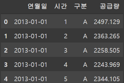

train.describe(include='all')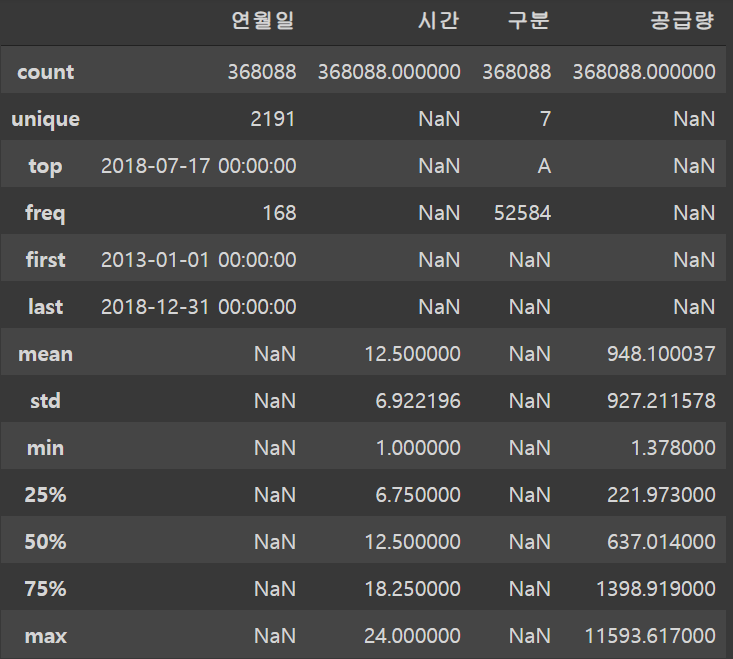

train.info()

<class 'pandas.core.frame.DataFrame'>
RangeIndex: 368088 entries, 0 to 368087
Data columns (total 4 columns):
 #   Column  Non-Null Count   Dtype         
---  ------  --------------   -----         
 0   연월일     368088 non-null  datetime64[ns]
 1   시간      368088 non-null  int64         
 2   구분      368088 non-null  object        
 3   공급량     368088 non-null  float64       
dtypes: datetime64[ns](1), float64(1), int64(1), object(1)
memory usage: 11.2+ MB

1.2.2 Testing Set

test.head()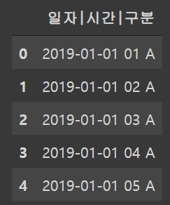

test.info()

<class 'pandas.core.frame.DataFrame'>
RangeIndex: 15120 entries, 0 to 15119
Data columns (total 1 columns):
 #   Column    Non-Null Count  Dtype 
---  ------    --------------  ----- 
 0   일자|시간|구분  15120 non-null  object
dtypes: object(1)
memory usage: 118.2+ KB

현제 Test set의 경우 세개의 변수들이 한개의 변수로 합쳐저있다.

1.3 데이터 변수 이름 변경

# Training set
train.columns = ["date", "hour", "class", "supply"]
## date: year-month-day
## hour: 시간
## class: 구분
## supply: 공급량

# Testing set
test.columns = ["DC"] 
## DC : date & class

print(train.head())
print(test.head())

        date  hour class    supply
0 2013-01-01     1     A  2497.129
1 2013-01-01     2     A  2363.265
2 2013-01-01     3     A  2258.505
3 2013-01-01     4     A  2243.969
4 2013-01-01     5     A  2344.105
                DC
0  2019-01-01 01 A
1  2019-01-01 02 A
2  2019-01-01 03 A
3  2019-01-01 04 A
4  2019-01-01 05 A

1.4 Training Set 전처리

변수 'date'를 'Year', 'Month', 'Day' 세개의 변수로 나누는게 좋을 수 있다.
요일 변수('weekday')를 추가하는게 좋을 것으로 보인다.

2013년 1월 1일은 화요일

def weekday(x):
    return x.weekday()

# date
train["year"] = train.date.apply(lambda x: x.year)
train["month"] = train.date.apply(lambda x: x.month)
train["day"] = train.date.apply(lambda x: x.day)
# Weekday
train["weekday"] = train.date.apply(weekday)

# Checking the missing value
np.sum(pd.isnull(train))

train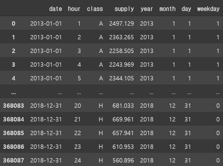

2 EDA

2.1 시간에 따른 가스공급량

plt.figure(figsize=(24, 8))
sns.lineplot(data=train, x="date", y="supply", ci=None)
plt.show()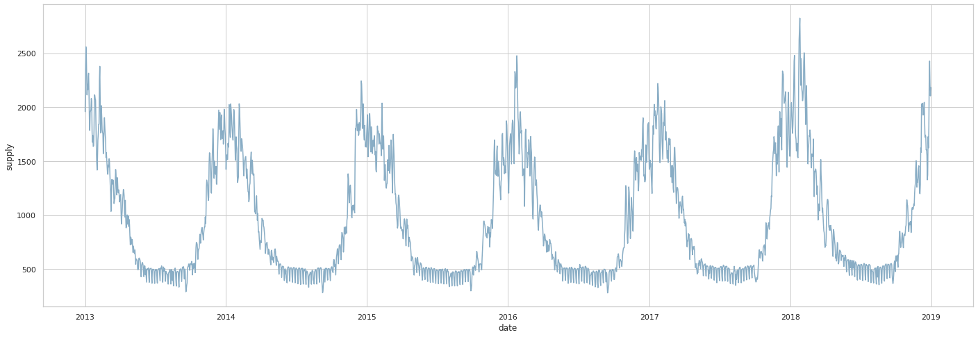

전체적인 흐름으로 봤을때 겨울에 가스공급량이 높게 나타난다.

온도에 따른 가스공급량 변화가 크게 변하는 것으로 추측된다.
2018년도에 가스공급량이 더욱 높게 나왔다.

2.1.1 연도에 따른 가스공급량

plt.figure(figsize=(12, 8))
sns.barplot(x="year", y="supply", data=train, label="total", color="b", ci=None)
plt.show()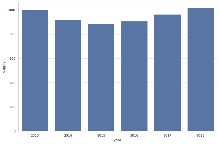

2013년도와 2018년도가 다른 해에 비해서 상대적으로 가스공급량이 많았다.
연도에 따른 가스공급량이 특정 트렌드를 보여주지는 않는다.

2.1.2 월에 따른 가스공급량

plt.figure(figsize=(12, 8))
## 월에 따른 그래프
plt.subplot(2, 1, 1)
sns.barplot(x="month", y="supply", data=train, 
            label="total", color="b", ci=None)
## 가스공급량순
plt.subplot(2, 1, 2)
order_list = train.groupby(["month"])['supply'].sum().sort_values().index
sns.barplot(x="month", y="supply", data=train, 
            label="total", color="b", ci=None, order=order_list)

plt.show()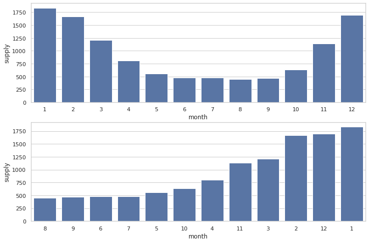

추운 계절이 있는 월에 가스공급량이 더 높게 나온다.
월에 대한 값또한 ordinial 형식으로 바꾸어 주는게 좋을 것으로 보인다.

2.1.3 요일에 따른 가스공급량

plt.figure(figsize=(12, 8))
sns.barplot(x="weekday", y="supply", data=train, 
            label="total", color="b", ci=None)
plt.show()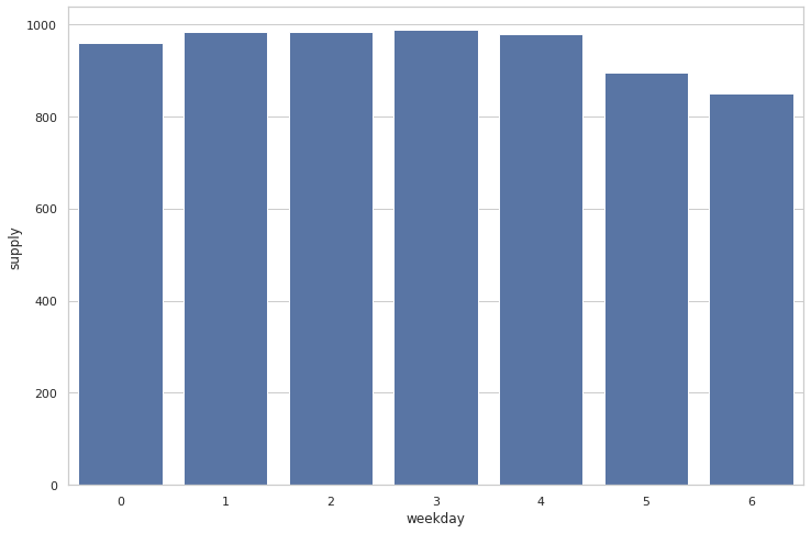

평일보다 주말에 가스공급량이 조금 낮게 나온다.

주말은 0 평일은 1로 마크해주는게 좋을것으로 보인다.

2.1.4 시간에 따른 가스공급량

plt.figure(figsize=(12, 8))
## 시간순
plt.subplot(2, 1, 1)
sns.barplot(x="hour", y="supply", data=train, 
            label="total", color="b", ci=None)
## 가스공급량순
order_list = train.groupby(["hour"])['supply'].sum().sort_values().index
plt.subplot(2, 1, 2)
sns.barplot(x="hour", y="supply", data=train, 
            label="total", color="b", ci=None, order=order_list)

plt.show()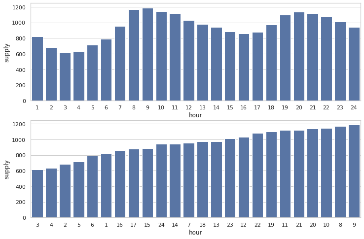

시간에 따른 공급량의 변화량을 보면 오전시간과 저녁시간에 사용량이 높게 나온다.
후에 모델링 전에 사용량이 적은 시간 부터 높은 시간으로 ordinial 순으로 적용하는 변환 시키는 것이 좋을 것으로 보인다.

2.2 구분에 따른 가스공급량

plt.figure(figsize=(12, 8))
## makes an order by gas usage
order_list = train.groupby(["class"])['supply'].sum().sort_values().index
sns.barplot(x="class", y="supply", data=train, 
            label="total", color="b", ci=None, order=order_list)
plt.show()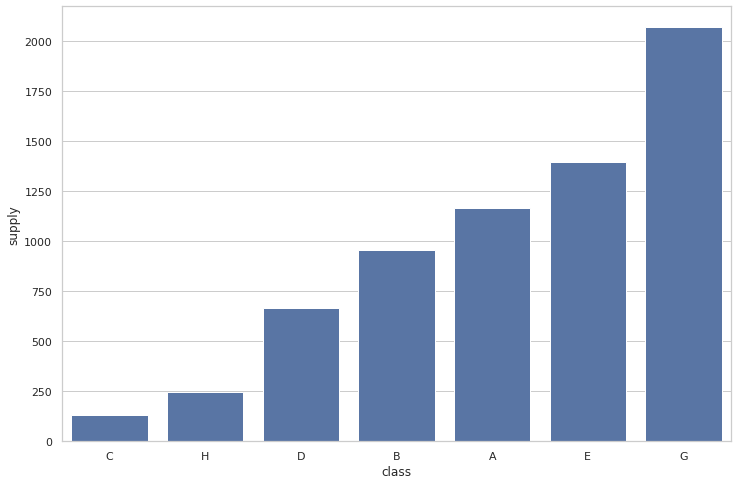

구분 별로 전체 가스공급량이 다르게 나타난다.

후에 one-hot 이 아닌 ordinial 형식으로 표현하는 것이 좋아보인다.

2.2.1 구분에 따른 요일별 가스공급량

plt.figure(figsize=(20, 10))

plt.subplot(2, 4, 1)
sns.barplot(x="weekday", y="supply", 
            data=train[train['class']=='A'], 
            label="total", color="b", ci=None)

plt.subplot(2, 4, 2)
sns.barplot(x="weekday", y="supply", 
            data=train[train['class']=='B'], 
            label="total", color="b", ci=None)

plt.subplot(2, 4, 3)
sns.barplot(x="weekday", y="supply", 
            data=train[train['class']=='C'], 
            label="total", color="b", ci=None)

plt.subplot(2, 4, 4)
sns.barplot(x="weekday", y="supply", 
            data=train[train['class']=='D'], 
            label="total", color="b", ci=None)

plt.subplot(2, 4, 5)
sns.barplot(x="weekday", y="supply", 
            data=train[train['class']=='E'], 
            label="total", color="b", ci=None)

plt.subplot(2, 4, 6)
sns.barplot(x="weekday", y="supply", 
            data=train[train['class']=='G'], 
            label="total", color="b", ci=None)

plt.subplot(2, 4, 7)
sns.barplot(x="weekday", y="supply", 
            data=train[train['class']=='H'], 
            label="total", color="b", ci=None)

plt.show()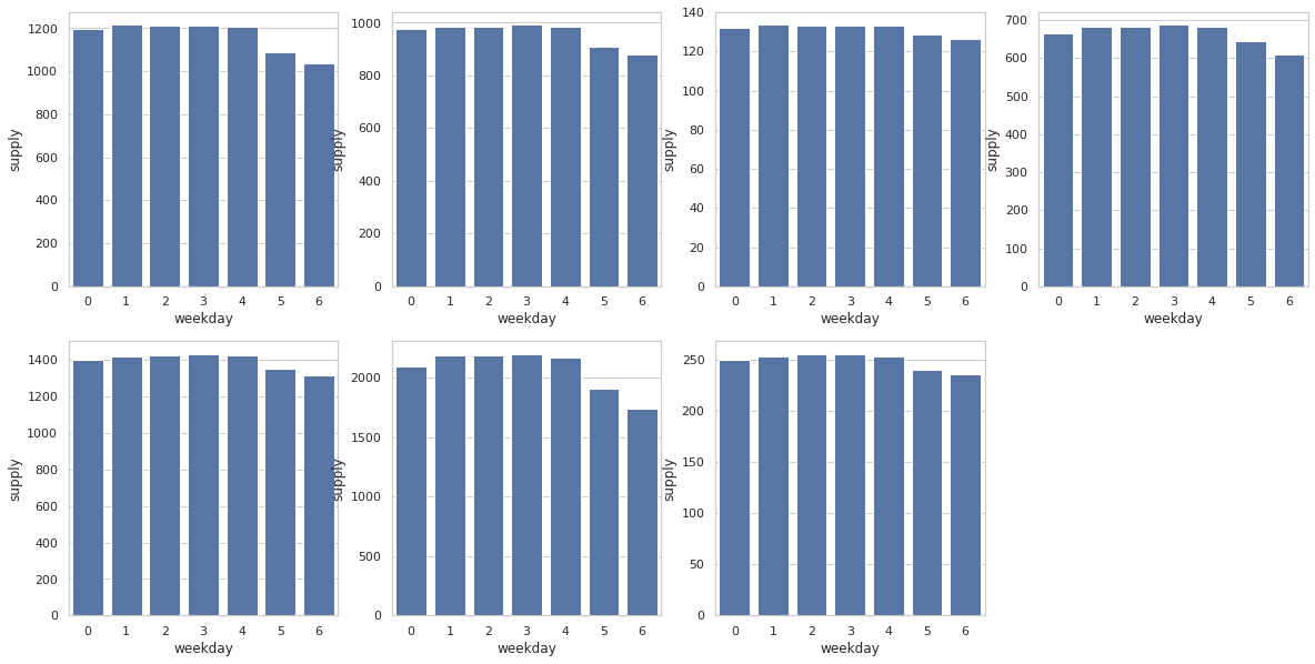

2.3 EDA 결과에 대한 토론

현재 데이터엔 feature에 대한 정보가 부족해 보인다.

따라서 추가적인 feature를 data sets에 join 시켜주는 것이 정확한 데이터 분석에 있어 좋을것으로 보인다.
가스 사용이 주로 이루어지는 부분은 난방, 온수, 요리 등 이 있다.
구분에 대해선 지역인 것으로 추측된다.

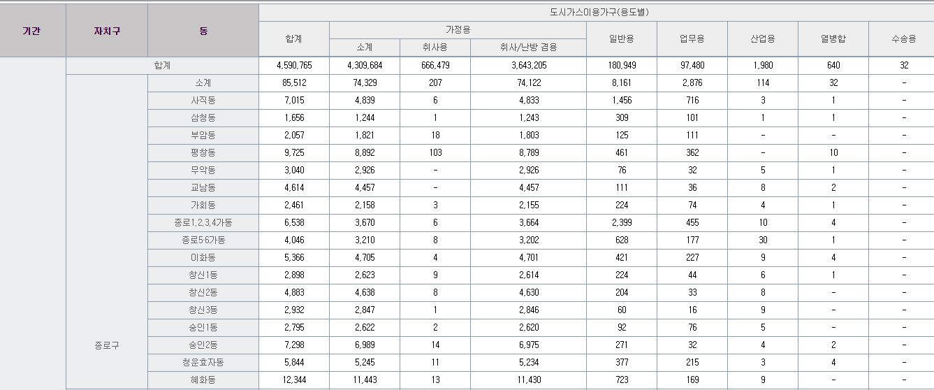
서울특별시 도시가스 이용현황

Link: https://data.seoul.go.kr/dataList/10120/S/2/datasetView.do

현재 표를 보면 가장 많은 가스 사용량은 '취사/난방 겸용'이다.

추가적인 feature엔 온도와 수도 사용량을 추가하는 것이 좋을 것으로 보인다.

구분 변수에 대한 정보가 부족하지만 지역별 가스 사용양일 것으로 추측된다.

국토교통부 시도별 에너지사용량

Link: https://www.molit.go.kr/USR/NEWS/m_71/dtl.jsp?id=95082347

지역별 도시가스, 전기, 지역난방 에너지사용량

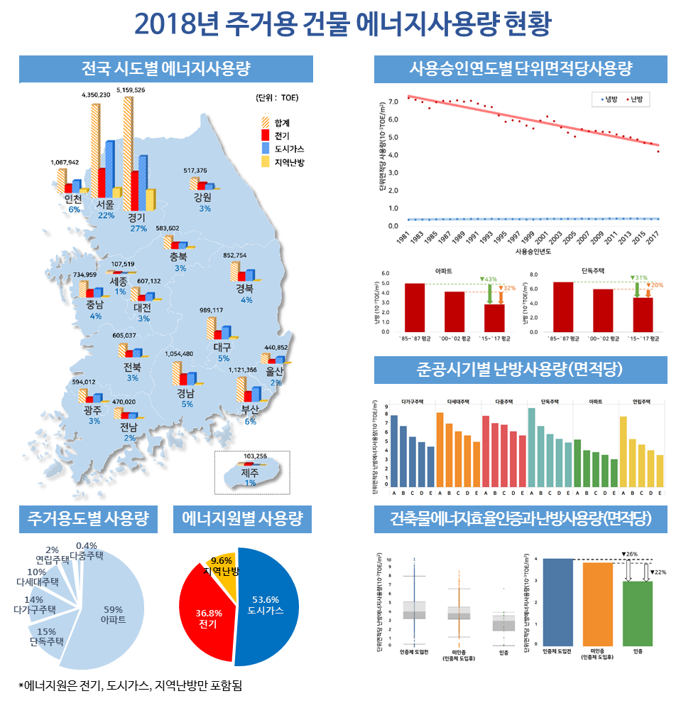
지역별 도시가스 사용량 비중

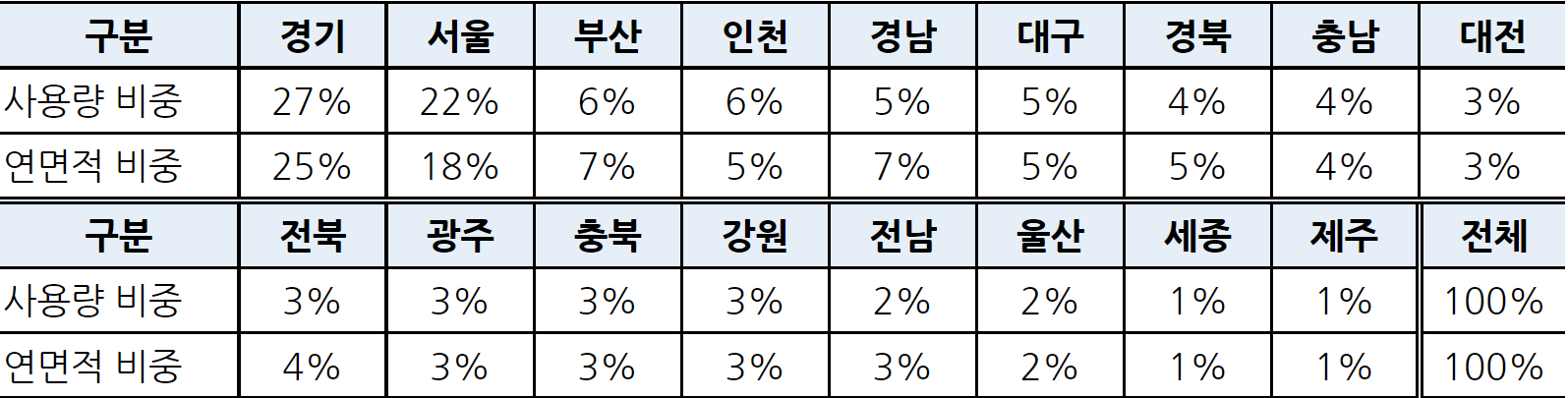
2018년 국토교통부에서 발표한 자료에 따르면 다음과 같은 비중으로 도시가스가 사용되었다.
위의 자료를 기준으로 변수 구분(class)에 대해 어느 정도 유추할 수 있을 것으로 생각된다.

데이터에서 2018년도 구분별 가스공급량 percentage

classes = train[train['year']==2018].groupby(['class']).agg({'supply': 'sum'})

class_supply_pcts = classes.apply(lambda x: 100*x/float(x.sum()))
class_supply_pcts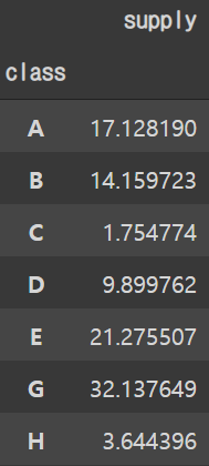

데이터에서 주어진 구분은 7개 임으로 위에 주어진 17개의 지역과 비교하기는 힘들것으로 보인다.

지역별 인구 및 인구밀도

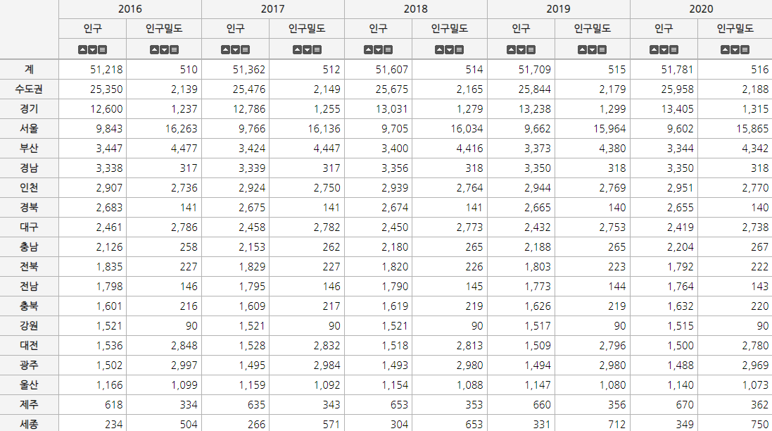
Link: https://www.index.go.kr/potal/main/EachDtlPageDetail.do?idx_cd=1007
나라지표

대한민국 행정구역

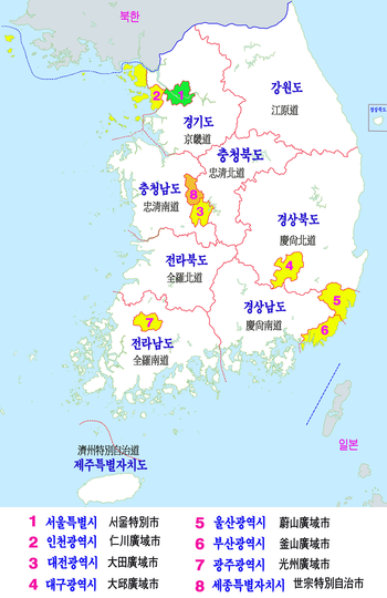
Link: https://ko.wikipedia.org/wiki/%EB%8C%80%ED%95%9C%EB%AF%BC%EA%B5%AD%EC%9D%98_%ED%96%89%EC%A0%95_%EA%B5%AC%EC%97%AD

인구수가 많으면 그에 따른 가스 사용량 또한 증가한다.
위에 보이는 지역별 인구수를 고려할 시 다음과 같이 지역을 예상 할 수 있다.

구분	예상되는 지역
G	경기도
E	서울
A	부산
B	인천
D	대구
H	울산
C	세종

3 날씨 데이터 처리

3.1 날씨 데이터 추가

EDA의 결과에 따르면 계절에 따라 가스공급량의 변화가 눈에 띄었다.

특희 겨울에 공급량이 높은걸로 보아 낮은온도에서 난방용으로 사용된 것으로 보인다.

날씨 데이터 추가

기상청 기상자료 개발포털에서 예상되는 지역에 대한 날씨 데이터를 시간별로 수집하였다.

종관기상관측(ASOS) 에서 기온, 강수량, 습도, 현지기압, 적설 변수를 가져왔다.

경기도의 경우 수원의 날씨를 사용하였다.

세종시의 경우 날씨데이터가 존재하지 않아 대전의 데이터를 가져왔다.

Link: https://data.kma.go.kr/data/grnd/selectAsosRltmList.do?pgmNo=36

# 날씨 데이터 기본 path 설정
base_path = "/content/drive/MyDrive/KDT/Project/5. 가스공급량/data/weather/"
# 날씨 데이터 지정
w2013 = pd.read_csv(base_path + "2013.csv", encoding='cp949', parse_dates=['일시'])
w2014 = pd.read_csv(base_path + "2014.csv", encoding='cp949', parse_dates=['일시'])
w2015 = pd.read_csv(base_path + "2015.csv", encoding='cp949', parse_dates=['일시'])
w2016 = pd.read_csv(base_path + "2016.csv", encoding='cp949', parse_dates=['일시'])
w2017 = pd.read_csv(base_path + "2017.csv", encoding='cp949', parse_dates=['일시'])
w2018 = pd.read_csv(base_path + "2018.csv", encoding='cp949', parse_dates=['일시'])
# 데이터 합치기
weather = pd.concat([w2013, w2014, w2015, w2016, w2017, w2018])

weather.head()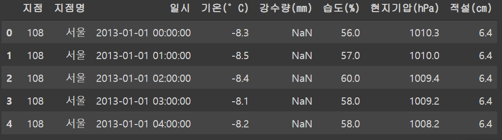

weather.info()

<class 'pandas.core.frame.DataFrame'>
Int64Index: 368060 entries, 0 to 61319
Data columns (total 8 columns):
 #   Column     Non-Null Count   Dtype         
---  ------     --------------   -----         
 0   지점         368060 non-null  int64         
 1   지점명        368060 non-null  object        
 2   일시         368060 non-null  datetime64[ns]
 3   기온(°C)     368056 non-null  float64       
 4   강수량(mm)    33440 non-null   float64       
 5   습도(%)      367862 non-null  float64       
 6   현지기압(hPa)  367714 non-null  float64       
 7   적설(cm)     8263 non-null    float64       
dtypes: datetime64[ns](1), float64(5), int64(1), object(1)
memory usage: 25.3+ MB

weather.describe(include='all')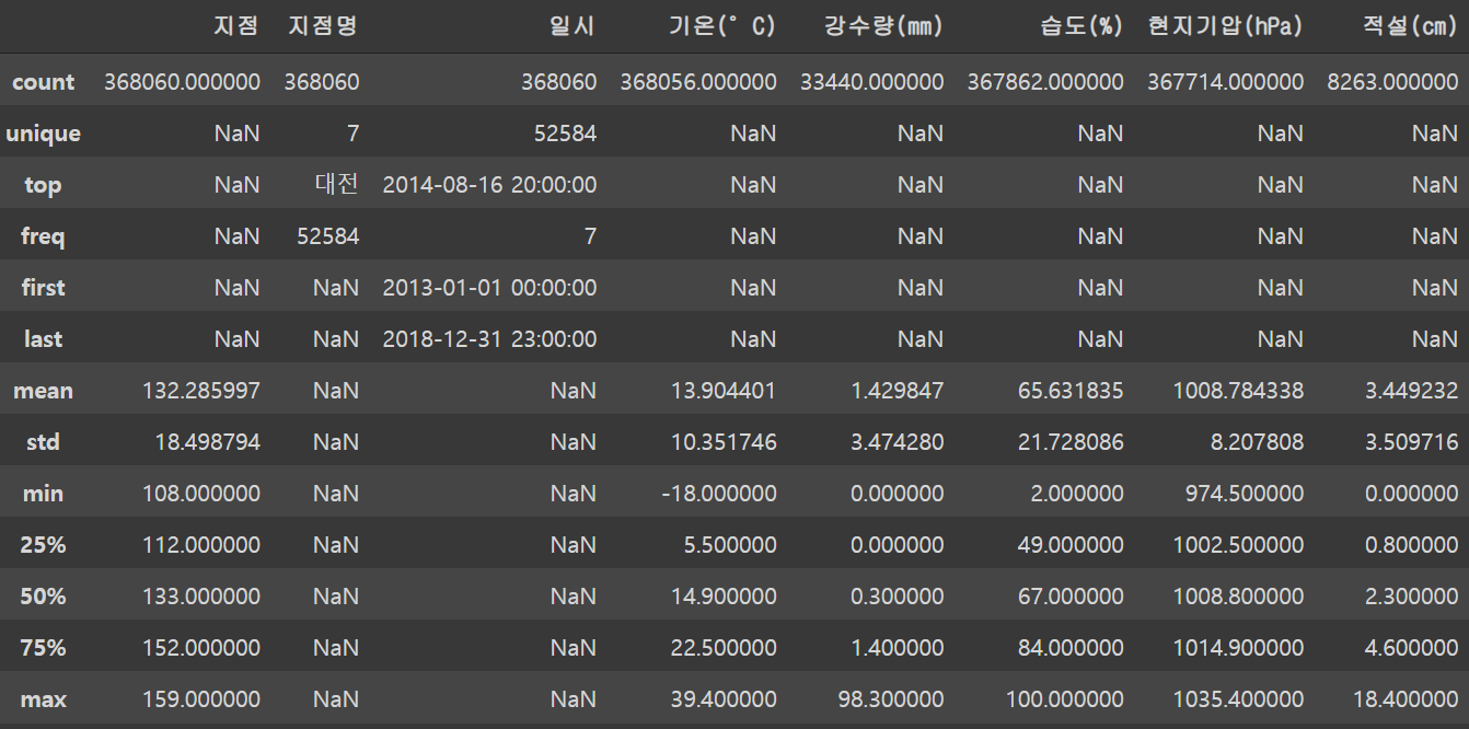

weather 데이터셋 column 변경사항

weather 데이터의 column의 이름을 변경한다.
Class의 지역 이름을 알파벳으로 변경한다.
현재 주어진 날씨 데이터에선 일시가 날짜와 시간이 합쳐져 있다.
Training set의 시간은 1, 2, 3, ..., 24 형식으로 되어있고 날씨 데이터의 경우 0, 1, 2, ..., 23 형식이다.

# column 이름 변경
weather.columns = ['point', 'class', 'dateTime', 'temperature',
                   'precipitation', 'humidity', 'pressure', 'snowdrifts']

pd.crosstab(weather['class'], weather['class'])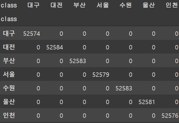

# class 값 변경
weather['class'][weather['class']=='부산'] = 'A'
weather['class'][weather['class']=='인천'] = 'B'
weather['class'][weather['class']=='대전'] = 'C'
weather['class'][weather['class']=='대구'] = 'D'
weather['class'][weather['class']=='서울'] = 'E'
weather['class'][weather['class']=='울산'] = 'H'
weather['class'][weather['class']=='수원'] = 'G'

## checking the result
pd.crosstab(weather['class'], weather['class'])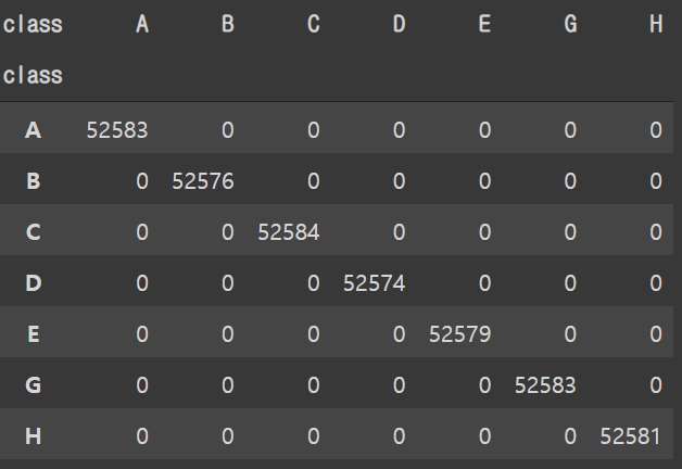

# 불필요한 column 버리기
weather.drop(columns=['point'], inplace=True)

weather.head()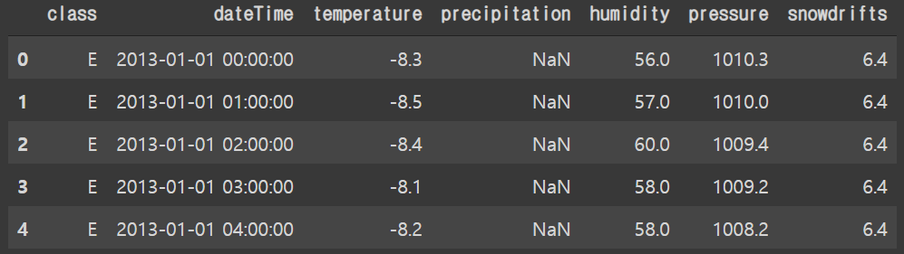

# 컬럼 순서 바꾸기
weather = weather[['dateTime', 'class', 'temperature',
                   'precipitation', 'humidity', 'pressure', 'snowdrifts']]

weather.head()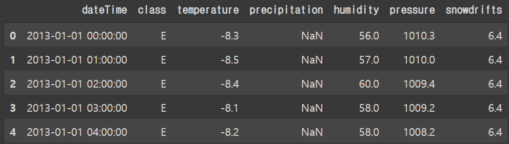

3.2 데이터 merge

training 과 weather를 merge 하기 위해선 dateTime 과 class 를 기준으로 해주어야 한다.

현재 weather 데이터의 경우 dateTime이 존재함으로 training set의 date 와 hour 값을 변경한다.

# 시간값 -1
train['hour'] = train['hour'] - 1
train['dateTime'] = train['date'] + pd.to_timedelta(train['hour'], unit='h')
# 원래대로 시간값 +1
train['hour'] = train['hour'] + 1

# training set column 순서 변경
train = train[['dateTime', 'class', 'date', 'hour', 
               'year', 'month', 'day', 'weekday', 'supply']]
train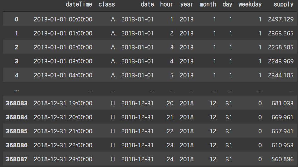

train = pd.merge(left=train, right=weather,
                 how='left', on=['dateTime', 'class'])

train.head()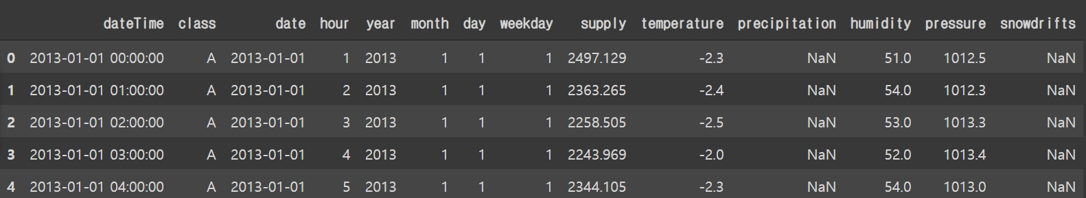

train.info()

<class 'pandas.core.frame.DataFrame'>
Int64Index: 368088 entries, 0 to 368087
Data columns (total 14 columns):
 #   Column         Non-Null Count   Dtype         
---  ------         --------------   -----         
 0   dateTime       368088 non-null  datetime64[ns]
 1   class          368088 non-null  object        
 2   date           368088 non-null  datetime64[ns]
 3   hour           368088 non-null  int64         
 4   year           368088 non-null  int64         
 5   month          368088 non-null  int64         
 6   day            368088 non-null  int64         
 7   weekday        368088 non-null  int64         
 8   supply         368088 non-null  float64       
 9   temperature    368056 non-null  float64       
 10  precipitation  33440 non-null   float64       
 11  humidity       367862 non-null  float64       
 12  pressure       367714 non-null  float64       
 13  snowdrifts     8263 non-null    float64       
dtypes: datetime64[ns](2), float64(6), int64(5), object(1)
memory usage: 42.1+ MB

3.3 결측값 처리

기존의 training set의 경우 결측값이 존재하지 않았으나 날씨데이터에는 결측값이 존재한다.

강수량(precipitation) 과 적설(snowdrifts)의 경우 결측값을 0으로 처리한다.

온도(temperature), 습도(humidity), 기압(pressure)에 대해선 interpolate을 사용하여 채워준다.

3.3.1 강수량과 적설 결측값 처리

train['precipitation'] = train['precipitation'].fillna(0)
train['snowdrifts'] = train['snowdrifts'].fillna(0)

train.info()

<class 'pandas.core.frame.DataFrame'>
Int64Index: 368088 entries, 0 to 368087
Data columns (total 14 columns):
 #   Column         Non-Null Count   Dtype         
---  ------         --------------   -----         
 0   dateTime       368088 non-null  datetime64[ns]
 1   class          368088 non-null  object        
 2   date           368088 non-null  datetime64[ns]
 3   hour           368088 non-null  int64         
 4   year           368088 non-null  int64         
 5   month          368088 non-null  int64         
 6   day            368088 non-null  int64         
 7   weekday        368088 non-null  int64         
 8   supply         368088 non-null  float64       
 9   temperature    368056 non-null  float64       
 10  precipitation  368088 non-null  float64       
 11  humidity       367862 non-null  float64       
 12  pressure       367714 non-null  float64       
 13  snowdrifts     368088 non-null  float64       
dtypes: datetime64[ns](2), float64(6), int64(5), object(1)
memory usage: 42.1+ MB

3.3.2 온도, 습도, 기압 결측값 처리

현재 데이터의 class는 alphabetical order를 따르고 있음으로 class 별로 묶어주어 interpolate해준다.

np.sum(pd.isnull(train))

dateTime           0
class              0
date               0
hour               0
year               0
month              0
day                0
weekday            0
supply             0
temperature       32
precipitation      0
humidity         226
pressure         374
snowdrifts         0
dtype: int64

train = train.groupby('class').apply(lambda x: x.interpolate())

np.sum(pd.isnull(train))

dateTime         0
class            0
date             0
hour             0
year             0
month            0
day              0
weekday          0
supply           0
temperature      0
precipitation    0
humidity         0
pressure         0
snowdrifts       0
dtype: int64

train.info()

<class 'pandas.core.frame.DataFrame'>
Int64Index: 368088 entries, 0 to 368087
Data columns (total 14 columns):
 #   Column         Non-Null Count   Dtype         
---  ------         --------------   -----         
 0   dateTime       368088 non-null  datetime64[ns]
 1   class          368088 non-null  object        
 2   date           368088 non-null  datetime64[ns]
 3   hour           368088 non-null  int64         
 4   year           368088 non-null  int64         
 5   month          368088 non-null  int64         
 6   day            368088 non-null  int64         
 7   weekday        368088 non-null  int64         
 8   supply         368088 non-null  float64       
 9   temperature    368088 non-null  float64       
 10  precipitation  368088 non-null  float64       
 11  humidity       368088 non-null  float64       
 12  pressure       368088 non-null  float64       
 13  snowdrifts     368088 non-null  float64       
dtypes: datetime64[ns](2), float64(6), int64(5), object(1)
memory usage: 52.1+ MB

3.4 날씨데이터 EDA

LGBM을 사용하여 성능을 확인한 결과 2013~2018년도의 날씨 데이터를 활용할 경우의 문제점이 발생하였다.

2013~2017년도의 날씨데이터를 활용하여 2018년도의 가스공급량을 예측하였을시 LGBR의 평균 MAE의 값이 1050 이상이 나왔다.

그러나 날씨데이터 활용 없이 예측하였을시 가장작은 MAE의 값이 264가 나왔다.

이번 대회에서 외부데이터의 사용시 문제점이 발생한다.
변수 구분이 무엇을 나타내는지 알 수 없음으로 해당 값에 어떠한 값을 넣어주어야 하는지 모른다.
변수 구분을 알고 있어도 training set을 활용하여 validation set의 추가한 변수에 대한 값을 예측해야한다.
예측된 변수(X) 값들로 가스공급량(y)을 제 예측하였을 시 정확성이 상대적으로 떨어질 수 밖에 없다.
따라서 외부데이터 사용시 해당 날짜에 해당 값을 삽입 하기보단 전체적으로 적용할 수 있는 값을 삽입하는 것이 좋을것으로 보인다.

# Compute the correlation matrix
corr = train.drop(columns=['hour', 'weekday', 'year', 'month', 'day']).corr()

# Generate a mask for the upper triangle
mask = np.triu(np.ones_like(corr, dtype=bool))

# Set up the matplotlib figure
f, ax = plt.subplots(figsize=(11, 9))

# Generate a custom diverging colormap
cmap = sns.diverging_palette(230, 20, as_cmap=True)

# Draw the heatmap with the mask and correct aspect ratio
sns.heatmap(corr, mask=mask, cmap=cmap, vmax=.3, center=0, annot=True,
            square=True, linewidths=.5, cbar_kws={"shrink": .5})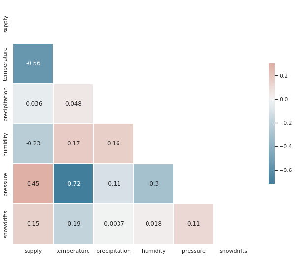

위의 Heatmap이 보여주는 값을 보면 날씨데이터 값들('precipitation'을 제외한)이 유의미한 연관성을 보여주고 있다.

model hyper paramater tunning에 있어 2013~2017년도의 날씨데이터를 training set으로 두고 2018년도의 데이터를 validation set으로 둔다.

Training and validation sets에 training set의 날씨데이터의 평균값을 넣어준다.

Hyper paramater tunning 완료 후 실제 testing set의 예측할 시 2014~2018년도의 데이터를 training set으로 두고 같은 방식으로 날씨데이터를 채워준다.

5 EDA 결과에 따른 Feature Engineering

5.1 구분(Class)

인구수가 많을수록 가스공급량 또한 증가한다.
가스공급량(supply)를 percentage로 나타내고 percentage 값을 가진 만단위의 인구수(pop_weight)를 생성한다.

classes = train.groupby(['class']).agg({'supply': 'sum'})

class_supply_pcts = classes.apply(lambda x: 100*x/float(x.sum()))
class_supply_pcts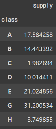

# pop_weight 생성
train['pop_weight'] = np.zeros(len(train))
# Weight 값 할당
train['pop_weight'][train['class']=='A'] = 1758
train['pop_weight'][train['class']=='B'] = 1444
train['pop_weight'][train['class']=='C'] = 198
train['pop_weight'][train['class']=='D'] = 1001
train['pop_weight'][train['class']=='E'] = 2102
train['pop_weight'][train['class']=='G'] = 3120
train['pop_weight'][train['class']=='H'] = 375

5.2 Month to Ordinial

plt.figure(figsize=(12, 5))

order_list = train.groupby(["month"])['supply'].sum().sort_values().index
sns.barplot(x="month", y="supply", data=train, 
            label="total", color="b", ci=None, order=order_list)

plt.show()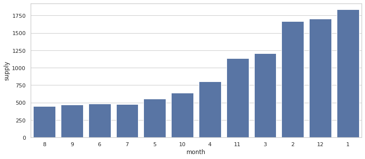

classes = train.groupby(['month']).agg({'supply': 'sum'})

class_supply_pcts = classes.apply(lambda x: 100*x/float(x.sum()))
class_supply_pcts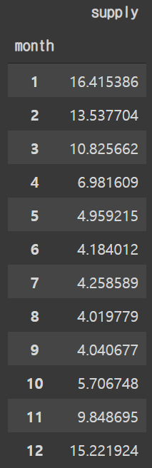

그래프와 표를 참고하여 m_weight을 만들어 사용한다.

표의 퍼센트 값 소숫점 한 자리에서 반올림 하여 m_weight값을 준다.

# m_weight 생성
train['m_weight'] = np.zeros(len(train))
# m_weight 값 할당
train['m_weight'][train['month']==1] = 16
train['m_weight'][train['month']==2] = 14
train['m_weight'][train['month']==3] = 11
train['m_weight'][train['month']==4] = 7
train['m_weight'][train['month']==5] = 5
train['m_weight'][train['month']==6] = 4
train['m_weight'][train['month']==7] = 4
train['m_weight'][train['month']==8] = 4
train['m_weight'][train['month']==9] = 4
train['m_weight'][train['month']==10] = 6
train['m_weight'][train['month']==11] = 10
train['m_weight'][train['month']==12] = 15

5.3 Hour to Ordinial

시간의 경우 사용량이 낮은 순에서 높은순으로 1 to 24 로 변환한다.

h_ord

plt.figure(figsize=(12, 8))

order_list = train.groupby(["hour"])['supply'].sum().sort_values().index
plt.subplot(2, 1, 2)
sns.barplot(x="hour", y="supply", data=train, 
            label="total", color="b", ci=None, order=order_list)

plt.show()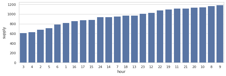

# h_ord 생성
train['h_ord'] = np.zeros(len(train))
# h_ord 값 할당
train['h_ord'][train['hour']==3] = 1
train['h_ord'][train['hour']==4] = 2
train['h_ord'][train['hour']==2] = 3
train['h_ord'][train['hour']==5] = 4
train['h_ord'][train['hour']==6] = 5
train['h_ord'][train['hour']==1] = 6
train['h_ord'][train['hour']==16] = 7
train['h_ord'][train['hour']==17] = 8
train['h_ord'][train['hour']==15] = 9
train['h_ord'][train['hour']==24] = 10
train['h_ord'][train['hour']==14] = 11
train['h_ord'][train['hour']==7] = 12
train['h_ord'][train['hour']==18] = 13
train['h_ord'][train['hour']==13] = 14
train['h_ord'][train['hour']==23] = 15
train['h_ord'][train['hour']==12] = 16
train['h_ord'][train['hour']==22] = 17
train['h_ord'][train['hour']==19] = 18
train['h_ord'][train['hour']==11] = 19
train['h_ord'][train['hour']==21] = 20
train['h_ord'][train['hour']==20] = 21
train['h_ord'][train['hour']==10] = 22
train['h_ord'][train['hour']==8] = 23
train['h_ord'][train['hour']==9] = 24

5.4 Weekday to 1

weekday_1: 평일을 1로 마킹한다.

# weekday_1 생성
train['weekday_1'] = np.zeros(len(train))
# h_ord 값 할당
train['weekday_1'][train['weekday']==0] = 1
train['weekday_1'][train['weekday']==1] = 1
train['weekday_1'][train['weekday']==2] = 1
train['weekday_1'][train['weekday']==3] = 1
train['weekday_1'][train['weekday']==4] = 1

6 데이터 저장

train.info()

<class 'pandas.core.frame.DataFrame'>
Int64Index: 368088 entries, 0 to 368087
Data columns (total 18 columns):
 #   Column         Non-Null Count   Dtype         
---  ------         --------------   -----         
 0   dateTime       368088 non-null  datetime64[ns]
 1   class          368088 non-null  object        
 2   date           368088 non-null  datetime64[ns]
 3   hour           368088 non-null  int64         
 4   year           368088 non-null  int64         
 5   month          368088 non-null  int64         
 6   day            368088 non-null  int64         
 7   weekday        368088 non-null  int64         
 8   supply         368088 non-null  float64       
 9   temperature    368088 non-null  float64       
 10  precipitation  368088 non-null  float64       
 11  humidity       368088 non-null  float64       
 12  pressure       368088 non-null  float64       
 13  snowdrifts     368088 non-null  float64       
 14  pop_weight     368088 non-null  float64       
 15  m_weight       368088 non-null  float64       
 16  h_ord          368088 non-null  float64       
 17  weekday_1      368088 non-null  float64       
dtypes: datetime64[ns](2), float64(10), int64(5), object(1)
memory usage: 63.4+ MB

# training set date to object
train.date = train.date.astype(str)
## checking the result
train.info()

<class 'pandas.core.frame.DataFrame'>
Int64Index: 368088 entries, 0 to 368087
Data columns (total 18 columns):
 #   Column         Non-Null Count   Dtype         
---  ------         --------------   -----         
 0   dateTime       368088 non-null  datetime64[ns]
 1   class          368088 non-null  object        
 2   date           368088 non-null  object        
 3   hour           368088 non-null  int64         
 4   year           368088 non-null  int64         
 5   month          368088 non-null  int64         
 6   day            368088 non-null  int64         
 7   weekday        368088 non-null  int64         
 8   supply         368088 non-null  float64       
 9   temperature    368088 non-null  float64       
 10  precipitation  368088 non-null  float64       
 11  humidity       368088 non-null  float64       
 12  pressure       368088 non-null  float64       
 13  snowdrifts     368088 non-null  float64       
 14  pop_weight     368088 non-null  float64       
 15  m_weight       368088 non-null  float64       
 16  h_ord          368088 non-null  float64       
 17  weekday_1      368088 non-null  float64       
dtypes: datetime64[ns](1), float64(10), int64(5), object(2)
memory usage: 63.4+ MB

base_path = "/content/drive/MyDrive/KDT/Project/5. 가스공급량/data/"
train.to_csv(base_path+'newTrain.csv', sep=',', index=False)

지리산근육곰