차원 & 차원 축소

현재 이미지는 100 * 100 = 10000개의 픽셀이 있다.
그래서 10000개의 특성을 가지고 있다고 볼 수 있으며, 이런 특성을 차원이라고 부른다.
이 차원을 줄이면 저장 공간을 크게 절약할 수 있다.

이런 비지도 학습 작업 중 하나가 차원 축소 알고리즘이다.

차원 축소는 데이터를 가장 잘 나타내는 특성들로만 이용하여 학습하는 방법으로, 작은 데이터로 비슷한 학습 성능을 낼 수 있다.

그리고 이런 차원 축소 알고리즘 중 대표적인 것이 주성분 분석(PCA)라고 한다.

주성분 분석

데이터에 있는 분산이 큰 방향을 찾는 것이다.

# n_components: 주성분 개수
pca = PCA(n_components=50)
pca.fit((fruits_2d))
print(pca.components_.shape)
# (50, 10000)

# 추출한 특성을 이용해서 그린 그림
draw_fruits(pca.components_.reshape(-1, 100, 100))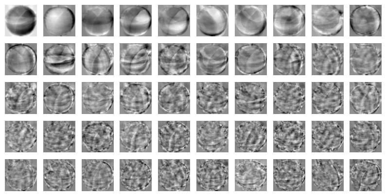

# 원본 데이터 크기
print(fruits_2d.shape)
# (300, 10000)

# 원본 데이터 차원 50으로 줄이기
# 50개의 특성을 가진 데이터
fruits_pca = pca.transform((fruits_2d))
print(fruits_pca.shape)
# (300, 50)

원본 데이터 재구성

그리고 inverse_transform()을 통해서 원본 데이터로 복원할 수 있다.

fruits_inverse = pca.inverse_transform(fruits_pca)
print(fruits_inverse.shape)
# (300, 10000)

그리고 이것을 그림으로 다시 출력하면

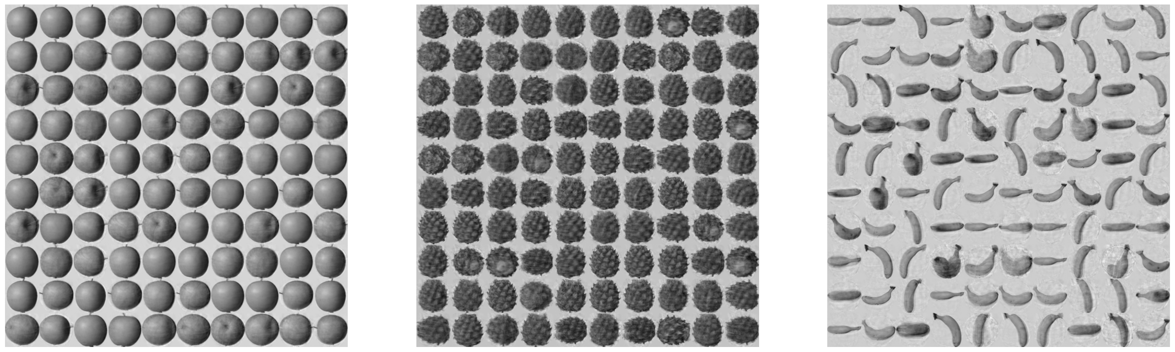
복원된것을 알 수 있다.

설명된 분산

주성분이 원본 데이터의 분산을 얼마나 잘 나타내는지 기록한 값을 설명된 분산이라고 한다.

explained_variance_ratio_에 분산 비율이 기록되어있다.

plt.plot(pca.explained_variance_ratio_)
plt.show()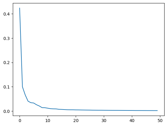

처음 10개의 성분으로 대부분을 표현하고 있다는 것을 알 수있다.

다른 알고리즘에 사용하기

로지스틱 회귀

from sklearn.linear_model import LogisticRegression
from sklearn.model_selection import cross_validate

lr = LogisticRegression()

target = np.array([0]*100 + [1]*100 + [2]*100)

# 로지스틱으로 일반적인 교차 검증
scores = cross_validate(lr, fruits_2d, target)
print(np.mean(scores['test_score']))
print(np.mean(scores['fit_time']))
# 0.9966666666666667
# 0.2760458469390869

scores = cross_validate(lr, fruits_pca, target)

# pca를 사용해 교차 검증
scores = cross_validate(lr, fruits_pca, target)
print(np.mean(scores['test_score']))
print(np.mean(scores['fit_time']))
# 0.9966666666666667
# 0.010817623138427735

50개의 특성만 사용했음에도 동일한 정확도가 나왔다.

# 개수 대신에 비율을 설정할 수 있다.
pca = PCA(n_components=0.5)
pca.fit(fruits_2d)

print(pca.n_components_)
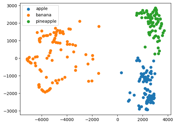
# 2

분산의 50%에 달하는 주성분 개수를 찾도록 설정할 수 있다.

해당 코드에서는 단 2개의 특성만으로 전체 분산의 50%를 설명할 수 있다는 것이다.

km = KMeans(n_clusters=3, random_state=42)
km.fit(fruits_pca)
print(np.unique(km.labels_, return_counts=True))
# (array([0, 1, 2], dtype=int32), array([110,  99,  91]))

앞의 결과와 비슷한 개수로 분류가 되었다.