import pandas as pd
import matplotlib.pyplot as plt
import matplotlib
import matplotlib.font_manager as fm
import seaborn as sns
import pandas as pd
from IPython.display import display
import numpy as np


pd.options.display.max_columns = None
%matplotlib inline

# 한글 폰트
plt.rcParams['font.family'] = 'NanumGothic'
# 마이너스 깨짐 방지
matplotlib.rcParams['axes.unicode_minus'] = False

# 나눔 폰트 경로 설정
font_path = '/usr/share/fonts/truetype/nanum/NanumGothic.ttf'  # 나눔 고딕의 경로
font_prop = fm.FontProperties(fname=font_path).get_name()

# 한글 폰트 설정
matplotlib.rcParams['font.family'] = font_prop

# 전역 팔레트 설정 (예: 'Set2' 팔레트 사용)
sns.set_palette('Set2')
sns_color = sns.color_palette('pastel')[0:5]
# 데이터 불러오기
regular_season = pd.read_csv('../datas/Regular_Season_Batter.csv')
regular_season_day = pd.read_csv('../datas/Regular_Season_Batter_Day_by_Day_b4.csv')
# 데이터프레임 null 값 확인
display(pd.DataFrame({'regular_season': regular_season.isna().sum(), 'regular_season_day': regular_season_day.isna().sum()}).fillna(''))
'''
앞서 각 데이터의 null 값을 모두 채웠기 때문에 없다.
첫 연봉은 제대로된 정보가 없고, 있더라도 조금씩 달라서 제외했다.
''';| regular_season | regular_season_day | |
|---|---|---|
| 2B | 0.0 | 0.0 |
| 3B | 0.0 | 0.0 |
| AB | 0.0 | 0.0 |
| BB | 0.0 | 0.0 |
| CS | 0.0 | 0.0 |
| E | 0.0 | |
| G | 0.0 | |
| GDP | 0.0 | 0.0 |
| H | 0.0 | 0.0 |
| HBP | 0.0 | 0.0 |
| HR | 0.0 | 0.0 |
| OBP | 0.0 | |
| OPS | 0.0 | |
| R | 0.0 | 0.0 |
| RBI | 0.0 | 0.0 |
| SB | 0.0 | 0.0 |
| SLG | 0.0 | |
| SO | 0.0 | 0.0 |
| TB | 0.0 | |
| avg | 0.0 | |
| avg1 | 0.0 | |
| avg2 | 0.0 | |
| batter_id | 0.0 | 0.0 |
| batter_name | 0.0 | 0.0 |
| career | 0.0 | |
| country | 0.0 | |
| date | 0.0 | |
| hand | 0.0 | |
| height/weight | 0.0 | |
| opposing_team | 0.0 | |
| pos | 0.0 | |
| position | 0.0 | |
| starting_salary | 1067.0 | |
| team | 0.0 | |
| year | 0.0 | 0.0 |
| year_born | 0.0 |
'''
입력된 데이터 중에서 잘못 입력된 데이터들이 있다.
그 데이터들을 수정했다.
수정하기 전에 각 컬럼이 어떤 것인지 다시 한 번 확인해 보았다.
''';
| 컬럼 이름 | 뜻 | 컬럼 이름 | 뜻 |
|---|---|---|---|
| batter_id | 타자 ID (고유 식별자) | HBP | 몸에 맞는 공 (Hit by Pitch) |
| batter_name | 타자 이름 | SO | 삼진 (Strikeouts) |
| year | 시즌 연도 | GDP | 병살타 (Grounded Into Double Play) |
| team | 소속 팀 이름 | SLG | 장타율 (Slugging Percentage, 총 루타 / 타수) |
| avg | 타율 (Batting Average, 안타 수 / 타수) | OBP | 출루율 (On-base Percentage, 출루 횟수 / 타석) |
| G | 경기 수 (Games Played) | E | 실책 수 (Errors) |
| AB | 타수 (At-Bats) | height/weight | 신장/체중 (Height/Weight) |
| R | 득점 (Runs Scored) | year_born | 출생 연도 (Year Born) |
| H | 안타 수 (Hits) | position | 포지션 (Position) |
| 2B | 2루타 (Doubles) | career | 경력 (Career, 몇 년 차인지) |
| 3B | 3루타 (Triples) | starting_salary | 연봉 (Starting Salary) |
| HR | 홈런 수 (Home Runs) | OPS | OPS (출루율 + 장타율, On-base Plus Slugging) |
| TB | 루타 수 (Total Bases) | pos | 세부 포지션 (Position Detail, 예: IF, OF 등) |
| RBI | 타점 (Runs Batted In) | hand | 타격/투구 손잡이 (Hand, 예: R-우타, L-좌타) |
| SB | 도루 (Stolen Bases) | country | 국적 (Country) |
| CS | 도루 실패 (Caught Stealing) | ||
| BB | 볼넷 (Base on Balls) |
'''
먼저 기존에 잘못 계산했기 때문에 잘못된 값이 들어가 있다.
그래서 값을 먼저 처음 값으로 되돌리고 진행한다.
'''
regular_season['SLG'] = pd.read_csv('../datas/62540_KBO_prediction_data/Regular_Season_Batter.csv', encoding='utf-8')['SLG']
regular_season['OBP'] = pd.read_csv('../datas/62540_KBO_prediction_data/Regular_Season_Batter.csv', encoding='utf-8')['OBP']
# 장타율 계산
# 안타는 1개 이상 있지만, 장타율이 0인 경우
display(regular_season[(regular_season['SLG'] == 0) & (regular_season['H'] > 0)].iloc[:, :22].head(3))
'''
SLG = (단타 + 2루타 *2 + 3루타 * 3 + 홈런 * 4) / 타수
SLG = H + (2B * 2) + (3B * 3) + (HR * 4) / AB
''';
# 장타율 계산
regular_season['SLG'] = regular_season.apply(lambda x: round(sum([x['H'], x['2B'] * 2, x['3B'] * 3, x['HR'] * 4]) / x['AB'], 3) if x['AB'] != 0 else 0, axis=1)
# 기존의 SLG과 새로 계산한 SLG
pd.concat(
[regular_season[['H', '2B', '3B', 'HR', 'AB']].map(int),
pd.read_csv('../datas/62540_KBO_prediction_data/Regular_Season_Batter.csv', encoding='utf-8')['SLG'].reset_index(drop=True), # 기존 SLG
regular_season['SLG'].reset_index(drop=True)], # 새로 계산한 SLG
axis=1 # 열 방향으로 병합
)| batter_id | batter_name | year | team | avg | G | AB | R | H | 2B | 3B | HR | TB | RBI | SB | CS | BB | HBP | SO | GDP | SLG | OBP | |
|---|---|---|---|---|---|---|---|---|---|---|---|---|---|---|---|---|---|---|---|---|---|---|
| 478 | 62 | 김주찬 | 2000 | 삼성 | 0.313 | 60 | 48 | 22 | 15 | 3 | 2 | 0 | 22 | 5 | 7 | 2 | 3 | 1 | 16 | 0 | 0.0 | 0.0 |
| 746 | 109 | 박기혁 | 2000 | 롯데 | 0.333 | 5 | 3 | 1 | 1 | 0 | 0 | 0 | 1 | 1 | 0 | 0 | 0 | 0 | 2 | 0 | 0.0 | 0.0 |
| 1457 | 207 | 이범호 | 2000 | 한화 | 0.162 | 69 | 74 | 11 | 12 | 7 | 0 | 1 | 22 | 3 | 1 | 0 | 10 | 1 | 21 | 2 | 0.0 | 0.0 |
| H | 2B | 3B | HR | AB | SLG | SLG | |
|---|---|---|---|---|---|---|---|
| 0 | 62 | 9 | 0 | 8 | 183 | 0.519 | 0.612 |
| 1 | 0 | 0 | 0 | 0 | 1 | 0.000 | 0.000 |
| 2 | 19 | 2 | 3 | 1 | 86 | 0.349 | 0.419 |
| 3 | 80 | 7 | 4 | 2 | 311 | 0.325 | 0.367 |
| 4 | 16 | 3 | 2 | 1 | 101 | 0.257 | 0.317 |
| ... | ... | ... | ... | ... | ... | ... | ... |
| 2449 | 0 | 0 | 0 | 0 | 5 | 0.000 | 0.000 |
| 2450 | 0 | 0 | 0 | 0 | 2 | 0.000 | 0.000 |
| 2451 | 0 | 0 | 0 | 0 | 10 | 0.000 | 0.000 |
| 2452 | 34 | 6 | 2 | 1 | 117 | 0.402 | 0.479 |
| 2453 | 4 | 1 | 0 | 1 | 24 | 0.333 | 0.417 |
2454 rows × 7 columns
# display(regular_season.head(2))
# OBP(출루율)
'''
OBP = (안타+볼넷+몸에 맞은 공)÷(타수+볼넷+몸에 맞은 공+희생플라이)
OBP = (H + BB + HBP) / (AB + BB + HBP + "") 이 데이터에는 희생플라이 컬럼이 없다.

그래서 문제가 있는 행은 제거한다.
'''

# 출루율이 잘못 입력되어있는 부분
drop_index = regular_season.loc[
    # 안타, 볼넷, 사구의 합이 0 이상인데 출루율이 0인 경우
    (sum([regular_season['H'] > 0, regular_season['BB'] > 0, regular_season['HBP']]) > 0) & (regular_season['OBP'] == 0) |
    # 타수, 볼넷, 사구의 합이 0 이상인데 출루율이 0인 경우
    (sum([regular_season['AB'] > 0, regular_season['BB'] > 0, regular_season['HBP']]) > 0) & (regular_season['OBP'] == 0)
    ].index

regular_season = regular_season.drop(drop_index).reset_index(drop=True)
regular_season.head(2)| batter_id | batter_name | year | team | avg | G | AB | R | H | 2B | 3B | HR | TB | RBI | SB | CS | BB | HBP | SO | GDP | SLG | OBP | E | height/weight | year_born | position | career | starting_salary | OPS | pos | hand | country | |
|---|---|---|---|---|---|---|---|---|---|---|---|---|---|---|---|---|---|---|---|---|---|---|---|---|---|---|---|---|---|---|---|---|
| 0 | 0 | 가르시아 | 2018 | LG | 0.339 | 50 | 183 | 27 | 62 | 9 | 0 | 8 | 95 | 34 | 5 | 0 | 9 | 8 | 25 | 3 | 0.612 | 0.383 | 9 | 177cm/93kg | 1985년 04월 12일 | 내야수(우투우타) | 쿠바 Ciego de Avila Maximo Gomez Baez(대) | NaN | 0.902 | 내야수 | 우타 | 외국인 |
| 1 | 1 | 강경학 | 2014 | 한화 | 0.221 | 41 | 86 | 11 | 19 | 2 | 3 | 1 | 30 | 7 | 0 | 0 | 13 | 2 | 28 | 1 | 0.419 | 0.337 | 6 | 180cm/72kg | 1992년 08월 11일 | 내야수(우투좌타) | 광주대성초-광주동성중-광주동성고 | 10000만원 | 0.686 | 내야수 | 좌타 | 한국인 |
# 규정타수 대비 OPS 시각화

plt.figure(figsize=(10, 5))
plt.plot('AB', 'OPS', data=regular_season, marker='o', linestyle='none', markersize=2, color='green', alpha=0.4)
plt.xlabel('AB(타수)', fontsize=14)
plt.ylabel('OPS(장타율)', fontsize=14)
# 규정 타수 30부터 OPS의 분포가 넓어졌기 때문에 30을 규정 타수로 정의하고 진행
plt.vlines(30, ymin=min(regular_season['OPS']), ymax=max(regular_season['OPS']), linestyles='dashed', colors='red')
plt.show()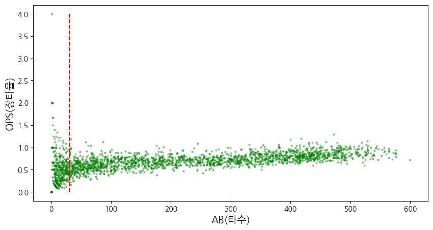
# OPS 이상치 탐색을 위한 수치 정의
Q1 = regular_season['OPS'].quantile(0.25)
Q3 = regular_season['OPS'].quantile(0.75)
IQR = Q3 - Q1

# print(f'{Q1 - 1.5 * IQR} < value < {Q3 + 1.5 * IQR}')

# 이상치 탐색
regular_season.loc[
    (regular_season['OPS'] < (Q1 - 1.5 * IQR))|
    (regular_season['OPS'] > (Q3 + 1.5 * IQR))
].sort_values(by=['AB'], axis=0, ascending=False)[['batter_name', 'AB', 'year', 'OPS']].head(10)| batter_name | AB | year | OPS | |
|---|---|---|---|---|
| 748 | 박병호 | 528 | 2015 | 1.150000 |
| 2212 | 테임즈 | 472 | 2015 | 1.293656 |
| 87 | 강정호 | 418 | 2014 | 1.200156 |
| 749 | 박병호 | 400 | 2018 | 1.175000 |
| 1253 | 유재신 | 33 | 2018 | 1.192000 |
| 2234 | 한승택 | 33 | 2013 | 0.165000 |
| 2046 | 채상병 | 32 | 2002 | 0.215909 |
| 391 | 김원섭 | 25 | 2005 | 0.116923 |
| 573 | 나주환 | 23 | 2013 | 0.174000 |
| 1469 | 이여상 | 22 | 2013 | 0.090909 |
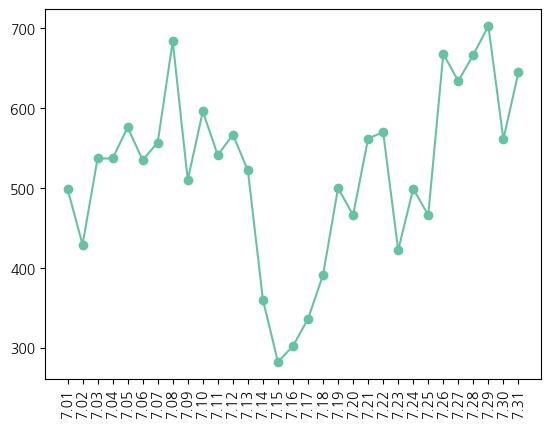
major_ticks = list(np.round(np.linspace(7.01, 7.31, 31), 2))

july = (regular_season_day['date'] >= 7) & (regular_season_day['date'] < 8)
plt.plot(major_ticks, regular_season_day['date'].loc[july].value_counts().sort_index(), marker='o')
plt.xticks(major_ticks, rotation=90)
plt.show()

코딩 공부하는 사람