import pandas as pd
import matplotlib.pyplot as plt
import matplotlib
import matplotlib.font_manager as fm
import seaborn as sns
import pandas as pd
from IPython.display import display
pd.options.display.max_columns = None
%matplotlib inline
plt.rcParams['font.family'] = 'NanumGothic'
matplotlib.rcParams['axes.unicode_minus'] = False
font_path = '/usr/share/fonts/truetype/nanum/NanumGothic.ttf'
font_prop = fm.FontProperties(fname=font_path).get_name()
matplotlib.rcParams['font.family'] = font_prop
sns.set_palette('Set2')
sns_color = sns.color_palette('pastel')[0:5]
regular_season_day = pd.read_csv('../datas/Regular_Season_Batter_Day_by_Day_b4.csv')
display(regular_season_day.head())
'''
매일의 데이터를 가지고 있다.
avg1은 해당 날짜의 타율, avg2는 총 타율을 의미한다.
opposing_team은 당시 상대팀을 의미한다.
''';
|
batter_id |
batter_name |
date |
opposing_team |
avg1 |
AB |
R |
H |
2B |
3B |
HR |
RBI |
SB |
CS |
BB |
HBP |
SO |
GDP |
avg2 |
year |
| 0 |
0 |
가르시아 |
3.24 |
NC |
0.333 |
3 |
1 |
1 |
0 |
0 |
0 |
0 |
0 |
0 |
1 |
0 |
1 |
0 |
0.333 |
2018 |
| 1 |
0 |
가르시아 |
3.25 |
NC |
0.000 |
4 |
0 |
0 |
0 |
0 |
0 |
0 |
0 |
0 |
0 |
0 |
1 |
0 |
0.143 |
2018 |
| 2 |
0 |
가르시아 |
3.27 |
넥센 |
0.200 |
5 |
0 |
1 |
0 |
0 |
0 |
0 |
0 |
0 |
0 |
0 |
0 |
0 |
0.167 |
2018 |
| 3 |
0 |
가르시아 |
3.28 |
넥센 |
0.200 |
5 |
1 |
1 |
0 |
0 |
0 |
1 |
0 |
0 |
0 |
0 |
0 |
0 |
0.176 |
2018 |
| 4 |
0 |
가르시아 |
3.29 |
넥센 |
0.250 |
4 |
0 |
1 |
0 |
0 |
0 |
3 |
0 |
0 |
0 |
0 |
0 |
1 |
0.190 |
2018 |
'''
date 열을 month, day로 분리한다.
'''
regular_season_day['month'] = regular_season_day['date'].apply(lambda x: str(x).split('.')[0])
regular_season_day['day'] = regular_season_day['date'].apply(lambda x: str(x).split('.')[1])
month_avg = regular_season_day.groupby(['year', 'month'])['avg2'].mean().reset_index()
month_avg_pivot = month_avg.pivot_table(index=['month'], columns=['year'], values=['avg2'])
display(month_avg_pivot)
'''
3월달과 10월달에만 결측치가 있는데, 이것은 3월에 시즌이 시작되고 10월쯤 시즌이 끝나기 때문에 있는 것 같다.
각 연도마다 시작과 끝 일정이 다르기 때문에 나타났다.
''';
|
avg2 |
| year |
2001 |
2002 |
2003 |
2004 |
2005 |
2006 |
2007 |
2008 |
2009 |
2010 |
2011 |
2012 |
2013 |
2014 |
2015 |
2016 |
2017 |
2018 |
| month |
|
|
|
|
|
|
|
|
|
|
|
|
|
|
|
|
|
|
| 10 |
0.356400 |
0.269065 |
0.216583 |
0.203636 |
NaN |
0.260985 |
0.249888 |
0.249638 |
0.033333 |
NaN |
0.243526 |
0.246949 |
0.257841 |
0.273537 |
0.274042 |
0.282547 |
0.280289 |
0.277482 |
| 3 |
NaN |
NaN |
NaN |
NaN |
NaN |
0.261714 |
0.261714 |
0.271982 |
NaN |
0.239861 |
NaN |
NaN |
0.231236 |
0.210598 |
0.214485 |
0.257857 |
0.161979 |
0.238015 |
| 4 |
0.205217 |
0.319792 |
0.250296 |
0.259663 |
0.235317 |
0.267106 |
0.215703 |
0.261531 |
0.252546 |
0.262953 |
0.247133 |
0.234199 |
0.267994 |
0.259918 |
0.255175 |
0.266711 |
0.259430 |
0.263953 |
| 5 |
0.297157 |
0.267990 |
0.241491 |
0.237954 |
0.253527 |
0.264283 |
0.237329 |
0.262535 |
0.280842 |
0.272934 |
0.250877 |
0.247844 |
0.268355 |
0.273899 |
0.261307 |
0.275240 |
0.274374 |
0.274083 |
| 6 |
0.306926 |
0.275867 |
0.252290 |
0.248800 |
0.249913 |
0.264392 |
0.260600 |
0.270766 |
0.278781 |
0.274791 |
0.263264 |
0.254577 |
0.270533 |
0.283480 |
0.268999 |
0.276307 |
0.279060 |
0.280630 |
| 7 |
0.293171 |
0.266650 |
0.244230 |
0.251973 |
0.256396 |
0.262464 |
0.259171 |
0.264870 |
0.275054 |
0.265501 |
0.264829 |
0.261513 |
0.262812 |
0.275677 |
0.272685 |
0.283192 |
0.284565 |
0.280817 |
| 8 |
0.303489 |
0.270481 |
0.252319 |
0.249460 |
0.243570 |
0.265369 |
0.270258 |
0.265173 |
0.271796 |
0.271075 |
0.262048 |
0.258069 |
0.268122 |
0.282025 |
0.272377 |
0.283105 |
0.283283 |
0.283923 |
| 9 |
0.308636 |
0.248333 |
0.243780 |
0.203953 |
0.237058 |
0.258794 |
0.251022 |
0.252942 |
0.264468 |
0.265312 |
0.258500 |
0.251232 |
0.260571 |
0.272411 |
0.271629 |
0.276513 |
0.273213 |
0.277841 |
'''
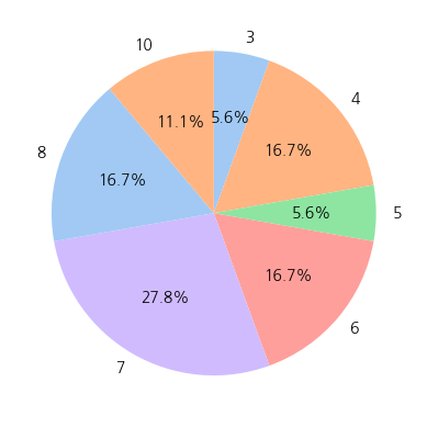
가장 높은 타율을 기록한 횟수가 가장 많은 달을 구해보려고 한다.
파이차트로 그려보려고 한다.
'''
best_avg_month = month_avg_pivot.idxmax().value_counts()
print(best_avg_month)
best_avg_month = {int(key): value for key, value in best_avg_month.to_dict().items()}
best_avg_month = dict(sorted(best_avg_month.items()))
display(best_avg_month)
best_avg_month_label = best_avg_month.keys()
best_avg_month_value = best_avg_month.values()
'''
startangle: 시작 기점(90 = 12시 방향)
counterclock: 어느 방향으로 데이터가 나열될 것인가(False = 시계 방향)
'''
plt.pie(best_avg_month_value, labels=best_avg_month_label, autopct='%.1f%%', startangle=90, colors=sns_color, counterclock=False)
plt.show()
7     5
8     3
4     3
6     3
10    2
3     1
5     1
Name: count, dtype: int64


{3: 1, 4: 3, 5: 1, 6: 3, 7: 5, 8: 3, 10: 2}
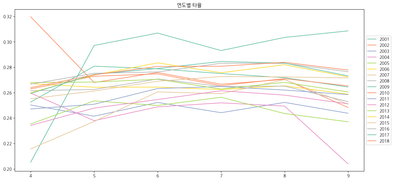
month_avg_rank_label = month_avg_pivot.mean().sort_values(ascending=False)[:3].index.get_level_values(1).to_numpy()
month_avg_rank_value = month_avg_pivot.mean().sort_values(ascending=False)[:3].values
print('평균 타율 순위')
for idx, (label, value) in enumerate(zip(month_avg_rank_label, month_avg_rank_value)):
print(f'{idx+1}st. {label}년: {value:.3f}')
print('----------')
month_best_avg_year = month_avg_pivot.idxmax()
month_best_avg_value = month_avg_pivot.max()
display(pd.DataFrame({
'최고 타율 연도': month_best_avg_year.map(lambda x: x+'월'),
'타율': month_best_avg_value
}).droplevel(0))
평균 타율 순위
1st. 2001년: 0.296
2st. 2016년: 0.275
3st. 2002년: 0.274
----------
|
최고 타율 연도 |
타율 |
| year |
|
|
| 2001 |
10월 |
0.356400 |
| 2002 |
4월 |
0.319792 |
| 2003 |
8월 |
0.252319 |
| 2004 |
4월 |
0.259663 |
| 2005 |
7월 |
0.256396 |
| 2006 |
4월 |
0.267106 |
| 2007 |
8월 |
0.270258 |
| 2008 |
3월 |
0.271982 |
| 2009 |
5월 |
0.280842 |
| 2010 |
6월 |
0.274791 |
| 2011 |
7월 |
0.264829 |
| 2012 |
7월 |
0.261513 |
| 2013 |
6월 |
0.270533 |
| 2014 |
6월 |
0.283480 |
| 2015 |
10월 |
0.274042 |
| 2016 |
7월 |
0.283192 |
| 2017 |
7월 |
0.284565 |
| 2018 |
8월 |
0.283923 |
display(month_avg_pivot.iloc[2:])
plt.figure(figsize=(15,7))
plt.plot(month_avg_pivot.iloc[2:])
plt.legend(month_avg_pivot.iloc[2:].columns.get_level_values(1), loc='center left', bbox_to_anchor=(1, 0.5))
plt.title('연도별 타율')
plt.show()
|
avg2 |
| year |
2001 |
2002 |
2003 |
2004 |
2005 |
2006 |
2007 |
2008 |
2009 |
2010 |
2011 |
2012 |
2013 |
2014 |
2015 |
2016 |
2017 |
2018 |
| month |
|
|
|
|
|
|
|
|
|
|
|
|
|
|
|
|
|
|
| 4 |
0.205217 |
0.319792 |
0.250296 |
0.259663 |
0.235317 |
0.267106 |
0.215703 |
0.261531 |
0.252546 |
0.262953 |
0.247133 |
0.234199 |
0.267994 |
0.259918 |
0.255175 |
0.266711 |
0.259430 |
0.263953 |
| 5 |
0.297157 |
0.267990 |
0.241491 |
0.237954 |
0.253527 |
0.264283 |
0.237329 |
0.262535 |
0.280842 |
0.272934 |
0.250877 |
0.247844 |
0.268355 |
0.273899 |
0.261307 |
0.275240 |
0.274374 |
0.274083 |
| 6 |
0.306926 |
0.275867 |
0.252290 |
0.248800 |
0.249913 |
0.264392 |
0.260600 |
0.270766 |
0.278781 |
0.274791 |
0.263264 |
0.254577 |
0.270533 |
0.283480 |
0.268999 |
0.276307 |
0.279060 |
0.280630 |
| 7 |
0.293171 |
0.266650 |
0.244230 |
0.251973 |
0.256396 |
0.262464 |
0.259171 |
0.264870 |
0.275054 |
0.265501 |
0.264829 |
0.261513 |
0.262812 |
0.275677 |
0.272685 |
0.283192 |
0.284565 |
0.280817 |
| 8 |
0.303489 |
0.270481 |
0.252319 |
0.249460 |
0.243570 |
0.265369 |
0.270258 |
0.265173 |
0.271796 |
0.271075 |
0.262048 |
0.258069 |
0.268122 |
0.282025 |
0.272377 |
0.283105 |
0.283283 |
0.283923 |
| 9 |
0.308636 |
0.248333 |
0.243780 |
0.203953 |
0.237058 |
0.258794 |
0.251022 |
0.252942 |
0.264468 |
0.265312 |
0.258500 |
0.251232 |
0.260571 |
0.272411 |
0.271629 |
0.276513 |
0.273213 |
0.277841 |