94일차 시작.... (앙상블 기법)

조동현·2022년 11월 22일

랜덤 포레스트 실습 랜덤 포레스트란?레이블 인코딩 작업 [레이블 인코딩]배깅(Bagging)이란?배깅과 부스팅의 공통점과 차이점 부스팅(boosting)이란?앙상블 기법 실습 앙상블 기법이란?원-핫 인코딩 작업 [레이블 인코딩]특성 중요도 추출

[교육] Python ML

목록 보기

9/17

📊 앙상블 기법

📌 앙상블 기법이란?

정의
- 개별적인 여러 모델들을 모아 종합적으로 취합 후, 최종 분류 결과를 출력하는 기법

종류
- voting : 직접투표, 간접투표
- bagging
- boosting

📌 앙상블 기법 실습

실습할 앙상블 모델
LogisticRegression + DecisionTree + KNN

1. 라이브러리 Import

import pandas as pd
import numpy as np
from sklearn.datasets import load_breast_cancer
from sklearn.model_selection import train_test_split

# 모델
from sklearn.linear_model import LogisticRegression
from sklearn.tree import DecisionTreeClassifier
from sklearn.neighbors import KNeighborsClassifier
from sklearn.ensemble import VotingClassifier

# 정확도 평가 지표
from sklearn.metrics import accuracy_score

2. 데이터 준비

# 2. 데이터 준비
breast = load_breast_cancer()
data = pd.DataFrame(breast.data, columns=breast.feature_names)
print(data.head(3))
#    mean radius  mean texture  ...  worst symmetry  worst fractal dimension
# 0        17.99         10.38  ...          0.4601                  0.11890
# 1        20.57         17.77  ...          0.2750                  0.08902
# 2        19.69         21.25  ...          0.3613                  0.08758

3. 학습, 테스트 데이터 분리

x_train, x_test, y_train, y_test = train_test_split(breast.data, breast.target, test_size=0.3, random_state=1)

print(x_train.shape, x_test.shape)
# (398, 30) (171, 30)

print(set(y_train))
# {0, 1}

4. 앙상블 모델에 사용할 개별 모델 준비

# 4. Ensemble 모델(VotingClassifier)
logi_model = LogisticRegression()
dt_model = DecisionTreeClassifier()
knn_model = KNeighborsClassifier(n_neighbors=3)

5. Ensemble 모델(VotingClassifier)
- estimators 속성 : 모델 지정
- voting 속성 : 투표 방법 지정
- hard voting : 다수결의 원칙으로 많이 표를 갖는 모델이 승리
- soft voting : 분류모델들의 분류 예측 확률값을 이용해 가장 높은 확률을 갖는 클래스를 예측함

ensemble = VotingClassifier(
	estimators=[('LR', logi_model), ('DT', dt_model), ('knn', knn_model)],
	voting='soft'
)

6. 개별 모델 학습 및 평가

classifiers = [logi_model, dt_model, knn_model]
for classifier in classifiers:
	# 개별 모델 학습
    classifier.fit(x_train, y_train)

    # 개별 모델 예측
    y_pred = classifier.predict(x_test)

    # 개별 모델 이름
    class_name = classifier.__class__.__name__

    # 개별 모델 정확도 출력
    print(f'{class_name} 모델 정확도 : ', accuracy_score(y_test, y_pred).round(3))
    # LogisticRegression 모델 정확도 :  0.924
    # DecisionTreeClassifier 모델 정확도 :  0.953
    # KNeighborsClassifier 모델 정확도 :  0.924

7. 앙상블 모델 학습 및 평가

ensemble.fit(x_train, y_train)
y_en_pred = ensemble.predict(x_test)
print('앙상블 모델 정확도 : ', accuracy_score(y_test, y_en_pred).round(3))
# 앙상블 모델 정확도 :  0.959

📊 앙상블 - Bagging, Boosting

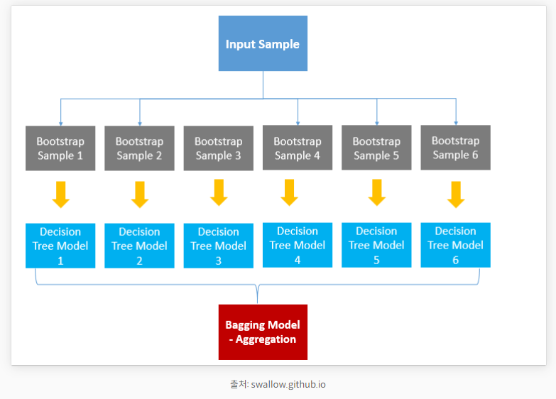
📌 배깅(Bagging)이란?

정의
- 배깅은 샘플을 여러 번 뽑아(Bootstrap) 각 모델을 학습시켜 결과물을 집계(Aggregration)하는 방법입니다
- Bagging = Bootstrap Aggregation

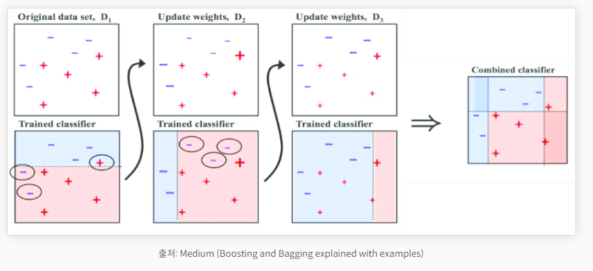
📌 부스팅(boosting)이란?

정의
- 부스팅은 가중치를 활용하여 약 분류기를 강 분류기로 만드는 방법
- 처음 모델이 예측을 하면 그 예측 결과에 따라 데이터에 가중치가 부여되고, 부여된 가중치가 다음 모델에 영향을 준다.

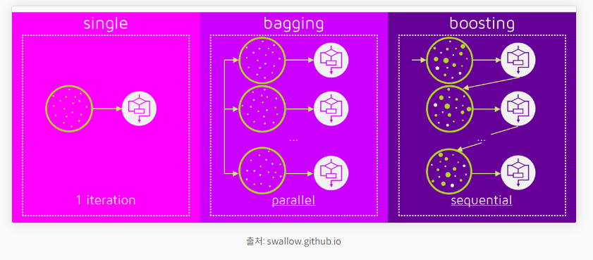
📌 배깅과 부스팅의 공통점과 차이점

차이점
- 배깅(bagging) : 병렬 처리
- 부스팅(boosting) : 직렬 처리

특징

- 배깅(bagging)의 예시 : 렌덤포레스트 모델
→ [ 밸런스 기반 ]

- 부스팅(boosting)의 예시 : XGboost 모델
→ [ 성능 기반 ]

공통점
- 두 기법 모두 여러 개의 모델을 사용하기 때문에 과적합을 주의해야 한다.

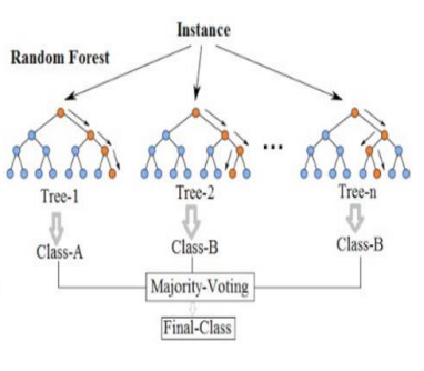
📊 랜덤 포레스트

📌 랜덤 포레스트란?

정의
- Random Forest는 ensemble(앙상블) Machine Learning 모델이다.
- 여러 개의 DecisionTree 사용
- 각 DecisionTree가 전체 데이터를 사용하는 것이 아닌 데이터 일부만 사용함 (Bagging)
- 각 트리가 분류한 결과에서 가장 많이 득표한 결과를 최종 분류 결과로 선택 (Ensemble Voting)

📌 랜덤 포레스트 실습

1. 라이브러리 Import

import pandas as pd
import numpy as np

# 레이블 인코딩 작업 : 라벨링 + 원-핫 인코딩
from sklearn.preprocessing import LabelEncoder, OneHotEncoder

from sklearn.model_selection import train_test_split
from sklearn.ensemble import RandomForestClassifier

2. 데이터 준비

# 타이타닉 데이터세트 사용
df = pd.read_csv("../testdata/titanic_data.csv")
print(df.head(3))
#    PassengerId  Survived  Pclass  ...     Fare Cabin  Embarked
# 0            1         0       3  ...   7.2500   NaN         S
# 1            2         1       1  ...  71.2833   C85         C
# 2            3         1       3  ...   7.9250   NaN         S

3. 결측치 확인

print(df.info())
# RangeIndex: 891 entries, 0 to 890
#  #   Column       Non-Null Count  Dtype  
# ---  ------       --------------  -----  
#  0   PassengerId  891 non-null    int64  
#  1   Survived     891 non-null    int64  
#  2   Pclass       891 non-null    int64  
#  3   Name         891 non-null    object 
#  4   Sex          891 non-null    object 
#  5   Age          714 non-null    float64
#  6   SibSp        891 non-null    int64  
#  7   Parch        891 non-null    int64  
#  8   Ticket       891 non-null    object 
#  9   Fare         891 non-null    float64
#  10  Cabin        204 non-null    object 
#  11  Embarked     889 non-null    object 

print(df.isnull().sum())
# PassengerId      0
# Survived         0
# Pclass           0
# Name             0
# Sex              0
# Age            177
# SibSp            0
# Parch            0
# Ticket           0
# Fare             0
# Cabin          687
# Embarked         2

3-1. 결측치 제거 후 사용 칼럼 추출

df = df.dropna(subset=['Pclass', 'Sex', 'Age'])
df = df.loc[:, ['Pclass', 'Sex', 'Age']]
print(df.info())
# Int64Index: 714 entries, 0 to 890
#  #   Column  Non-Null Count  Dtype  
# ---  ------  --------------  -----  
#  0   Pclass  714 non-null    int64  
#  1   Sex     714 non-null    object 
#  2   Age     714 non-null    float64

4-1. 레이블 인코딩 작업 [레이블 인코딩]
- ⭐ LabelEncoder 모듈 : Number 라벨링

# 1) 레이블 라벨링 작업
encoder = LabelEncoder()
df['Sex'] = encoder.fit_transform(df['Sex'])
print(df.head(2))
#    Pclass  Sex   Age
# 0       3    1  22.0
# 1       1    0  38.0

4-2. 원-핫 인코딩 작업 [레이블 인코딩]
- ⭐ OneHotEncoder 모듈 : 범주형 데이터 값을 0과 1을 사용하여 표현

onehot = OneHotEncoder()
print(onehot.fit_transform(df[['Pclass']]).toarray())
# [[0. 0. 1.]
#  [1. 0. 0.]
#  [0. 0. 1.]
#  ...
#  [1. 0. 0.]
#  [1. 0. 0.]
#  [0. 0. 1.]]

df_onehot = pd.DataFrame(onehot.fit_transform(df[['Pclass']]).toarray())
df_onehot.columns = ['f_class', 's_class', 't_class']
df = pd.concat([df, df_onehot], axis=1)
print(df.head(2))
#    Pclass  Sex   Age  Survived  f_class  s_class  t_class
# 0     3.0  1.0  22.0       0.0      0.0      0.0      1.0
# 1     1.0  0.0  38.0       1.0      1.0      0.0      0.0

5. 학습, 테스트 데이터 분리

df_x = df.drop(['Survived'], axis=1)
df_y = df['Survived']
x_train, x_test, y_train, y_test = train_test_split(df_x, df_y, test_size=0.3, random_state=1)
print(x_train.shape, x_test.shape, y_train.shape, y_test.shape)
# (602, 6) (259, 6) (602,) (259,)

6. 랜덤 포레스트 모델

model = RandomForestClassifier(n_estimators=500, criterion='entropy')
model.fit(x_train, y_train)

7. 예측값, 실제값 비교

y_pred = model.predict(x_test)
print('실제값 : ', np.array(y_test[:3]))
print('예측값 : ', y_pred[:3])
# 실제값 :  [1. 0. 0.]
# 예측값 :  [0. 0. 0.]

8. 성능 평가

print('acc : ', accuracy_score(y_test, y_pred))
# acc :  0.783625730994152

9. 교차 검증

cross_val = cross_val_score(model, df_x, df_y, cv=5)
print(cross_val)
print(np.mean(cross_val))
# [0.74561404 0.79824561 0.81415929 0.78761062 0.79646018]
# 0.7884179475236764

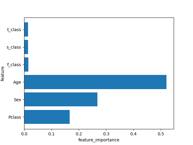
10. 특성 중요도 추출

print('특정(변수) 중요도 : ', model.feature_importances_)
# 특정(변수) 중요도 :  [0.16178083 0.26556737 0.52703405 0.01613185 0.01424291 0.01524298]

def plot_importance(model):
    n_features = df_x.shape[1]
    plt.barh(np.arange(n_features), model.feature_importances_)
    plt.yticks(np.arange(n_features), df_x.columns)
    plt.xlabel('feature_importance')
    plt.ylabel('feature')
    plt.show()

plot_importance(model)