93일차 시작.... (결정 트리)
Python 결정트리 그래프 출력 선행 모듈 설치sklearn Decision Tree 모델결정 트리란?과적합 방지 방법1 - train_test_split과적합 방지 방법2 - 교차검증(cross validation)과적합 방지 방법3 - 교차검증 모듈 사용 (cross_val_score)혼잡도/불순도란?
[교육] Python ML
목록 보기
8/17

📊 분류 분석 - Decision Tree
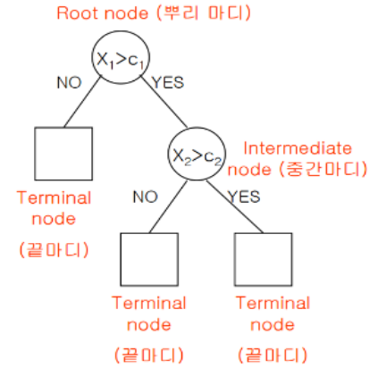
📌 결정 트리란?
- 정의
- 여러가지 규칙을 순차적으로 독립 변수 공간을 분리하며 자식 노드의 혼잡도(불순도)가 낮아질 때까지 분류한다.
📌 혼잡도/불순도란?
- 정의
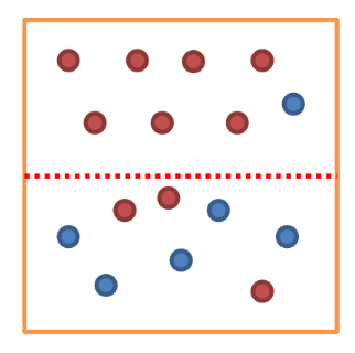
- 결정 트리의 각 노드에서 여러 독립변수가 혼잡된 수치
- 혼잡도 지표
- Entorpy
- Gini 계수
📌 Python 결정트리 그래프 출력 선행 모듈 설치
- 절차
1) graphviz 설치
2) 설치 후 graphviz 폴더의 bin 폴더로 이동
3) 경로 복사
4) 고급 시스템 설정 보기 → 환결 설정 → path 수정
5) 경로 붙여넣기 → path 수정 완료
6) anaconda prompt 실행
7) pip install graphviz
8) pip install pydotplus
📊 sklearn Decision Tree 모델
📌 결정트리 모델 학습
- 1. 라이브러리 Import
import pydotplus
from sklearn import tree
import collections
- 2. 데이터 준비
x = [[180, 15], [177, 42], [156, 35], [174, 5], [166, 33]]
y = ['man', 'woman', 'woman', 'man', 'woman']
label_names = ['height', 'hair Length']
- 3. 모델 학습
criterion 속성 : 노드의 독립변수 혼잡도를 측정할 지표를 설정
max_depth 속성 : 결정트리의 최대 깊이를 설정
min_samples_split 속성 : 노드 분할을 위한 최소 표본수 제어 값model = tree.DecisionTreeClassifier( criterion='entropy', max_depth=2, min_samples_split= random_state=0 ) model.fit(x, y)
- 4. 모델 성능 평가
print('훈련 정확도 : ', model.score(x, y))
# 훈련 정확도 :  1.0
- 5. 예측값, 실제값 비교
print('예측값 : ', model.predict(x))
print('실제값 : ', y)
# 예측값 :  ['man' 'woman' 'woman' 'man' 'woman']
# 실제값 :  ['man', 'woman', 'woman', 'man', 'woman']
- 6. 실제 예측하기
mydata = [[171, 78]]
new_pred = model.predict(mydata)
print(new_pred)
# ['woman']
- 7. 결정트리 시각화
dot_data = tree.export_graphviz(model, feature_names=label_names, out_file=None, filled=True, rounded=True)
graph = pydotplus.graph_from_dot_data(dot_data)
colors = ('red', 'blue')
edges = collections.defaultdict(list)

for e in graph.get_edge_list():
    edges[e.get_source()].append(int(e.get_destination()))

for e in edges:
    edges[e].sort()
    for i in range(2):
        dest = graph.get_node(str(edges[e][i]))[0]
        dest.set_fillcolor(colors[i])

graph.write_png('tree.png')
- 8. 저장한 이미지 읽기
img = imread('tree.png')
plt.imshow(img)
plt.show()
📊 과적합 방지 방법
📌 과적합 방지 방법1 - train_test_split
- 학습, 테스트 데이터 분리
- 데이터세트 하나로 학습하고 테스트하게 되면 과적합을 발생시킨다.
- 데이터세트를 학습데이터와 테스트데이터로 분리하여 용도에 맞게 학습 및 테스트하여 과적합을 해소한다.from sklearn.model_selection import train_test_split x_train, x_test, y_train, y_test = train_test_split(train_data, train_label, test_size=0.3, random_state=1) print(x_train.shape, x_test.shape) # (105, 4) (45, 4) # 훈련데이터로 모델 학습 model = DecisionTreeClassifier() model.fit(x_train, y_train) y_pred = model.predict(x_test) print('테스트 정확도 : ', accuracy_score(y_pred, y_test)) # 테스트 정확도 : 0.9555555555555556
📌 과적합 방지 방법2 - 교차검증(cross validation)
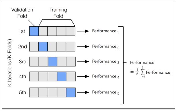
- 교차 검증(Cross Validation)
- 학습, 테스트 데이터로 분리해도 과적합이 발생된다면 검증데이터 사용 고려
- 분리한 학습데이터에서 일부를 검증데이터로 사용한다.
- 전체 학습데이터 = 일부 학습데이터 + 검증데이터
- 교차검증은 모델 학습 도중에 k번 학습데이터에서 검증데이터를 분리하여 학습 시 검증도 함께 수행한다.
[ 과적합 발생시 교차검증 ]
1) 필요 라이브러리
from sklearn.model_selection import KFold
import numpy as np
2) 데이터 준비
features = iris.data
label = iris.target
3) KFold 객체 준비
kfold = KFold(n_splits=5)
4) KFold를 이용해 학습, 검증 데이터 분할 (교차검증)
n_iter = 0		# KFold 실행 순번 저장
n_acc = []		# 각 모델의 정확도 저장
for train_index, test_index in kfold.split(features):
    n_iter += 1

    # 학습, 검증 데이터 분할
    x_train, x_test = features[train_index], features[test_index]
    y_train, y_test = label[train_index], label[test_index]

    # 분리된 학습데이터로 모델 학습
    model.fit(x_train, y_train)

    # 각 모델 정확도 평가
    y_pred = model.predict(x_test)
    print(f'{n_iter}번째 모델 정확도 : ', accuracy_score(y_test, y_pred))
    # 1번째 모델 정확도 :  1.0
    # 2번째 모델 정확도 :  0.9666666666666667
    # 3번째 모델 정확도 :  0.9
    # 4번째 모델 정확도 :  0.9333333333333333
    # 5번째 모델 정확도 :  0.8

	# 각 모델의 정확도 저장
    n_acc.append(accuracy_score(y_test, y_pred))
5) 평균 정확도 계산
print('평균 정확도 : ', np.mean(n_acc))
# 평균 정확도 :  0.9199999999999999
[ 불균형한 분포(평향, 왜곡) 발생시 교차검증 ]
→ 불균형이란 특정 레이블 값이 특이하게 많거나 적은 경우
1) 필요 라이브러리
from sklearn.model_selection import StratifiedKFold
2) 데이터 준비
features = iris.data
label = iris.target
3) KFold 객체 준비
skfold = StratifiedKFold(n_splits=5)
4) KFold를 이용해 학습, 검증 데이터 분할 (교차검증)
n_iter = 0		# KFold 실행 순번 저장
n_acc = []		# 각 모델의 정확도 저장
for train_index, test_index in skfold.split(features, label):
    n_iter += 1

    # 학습, 검증 데이터 분할
    x_train, x_test = features[train_index], features[test_index]
    y_train, y_test = label[train_index], label[test_index]

    # 분리된 학습데이터로 모델 학습
    model.fit(x_train, y_train)

    # 각 모델 정확도 평가
    y_pred = model.predict(x_test)
    print(f'{n_iter}번째 모델 정확도 : ', accuracy_score(y_test, y_pred))
    # 1번째 모델 정확도 :  0.9666666666666667
    # 2번째 모델 정확도 :  0.9666666666666667
    # 3번째 모델 정확도 :  0.9
    # 4번째 모델 정확도 :  0.9333333333333333
    # 5번째 모델 정확도 :  1.0

	# 각 모델의 정확도 저장
    n_acc.append(accuracy_score(y_test, y_pred))
5) 평균 정확도 계산
print('평균 정확도 : ', np.mean(n_acc))
# 평균 정확도 :  0.9533333333333334
📌 과적합 방지 방법3 - 교차검증 모듈 사용 (cross_val_score)
- cross_val_score 모듈
- KFold 교차검증 지원하는 모듈
- 1. 필요 라이브러리
from sklearn.model_selection import cross_val_score
- 2. 데이터 준비
data = iris.data
label = iris.target
- 3. 모델 준비
model = DecisionTreeClassifier(criterion='entropy', random_state=1)
- 4. 교차검증 수행
- estimator 속성 : 정의한 모델 지정
- X 속성 : 학습 features 지정
- y 속성 : 학습 label 지정
- scoring 속성 : 성능 평가 방법 지정
- cv 속성 : KFold의 k개를 지정score = cross_val_score(model, data, label, scoring='accuracy', cv=5)
- 5. 모델 정확도 평가
print('교차 검증별 정확도 : ', score)
print('평균 검증 정확도 : ', np.mean(score))
# 교차 검증별 정확도 :  [0.96666667 0.96666667 0.9 0.93333333 1.]
# 평균 검증 정확도 :  0.9533333333333334

데이터 사이언티스트를 목표로 하는 개발자