Tacotron: Towards End-to-End Speech Synthesis
paper: https://arxiv.org/pdf/1703.10135
audio sample: https://google.github.io/tacotron/publications/tacotron/index.html
code: [original - tf] https://github.com/keithito/tacotron/blob/master/models/tacotron.py
[torch] https://github.com/r9y9/tacotron_pytorch/blob/master/tacotron_pytorch/tacotron.py
작성
[참고] https://khw11044.github.io/blog/papers/paper-etc/2021-01-31-tacotron1_summary/
ABSTRACT
- TTS시스템 : 전형적으로 text analysis frontend, acoustic model, audio 합성 모듈과 같은 multiple stage의 시스템이다.
- 이러한 것들은 특정 도메인의 전문지식이 요구되고 불안정한 디자인을 선택하였다.
- 이 논문에서 Character로부터 직접 음성을 합성하는 end-to-end TTS 모델인 Tacotron을 제안한다.
- <text, audio> pair 주어지면, 이 모델은 랜덤 초기화 이후 처음부터 완벽하게 학습될수 있다.
- Sequence-to-sequence 프레임워크가 이 어려운 태스크를 위해 잘 동작하기 위한 몇가지 중요한 테크닉들을 제안한다.
- Tacotron은 미국 영어를 타겟으로 5점 만점의 mean opinion score에서 3.82점에 도달하였다. 자연스러움에서 기존 parametric system을 능가한다.
- 게다가, Tacotron은 프레임 수준에서 음성을 생성하기 때문에, 샘플 수준의 autoregressive 방법들보다 빠르다.
1 INTRODUCTION
기존 방법들의 문제점
- 현대 TTS 파이프라인은 복잡함. 전문적인 지식을 기반으로 하고 디자인하기 매우 어려움
- 1) 다양한 언어학적 특성들을 추출하는 text frontend
- 2) 음성 길이를 예측하는 모델
- 3) 음성 특성을 예측하는 모델
- 4) 복잡한 signal processing 기반의 vocoder

- 파이프라인의 각 component들 개별적으로 학습되기 때문에, 컴포넌트 별 에러들 축적됨.
End-to-end TTS 시스템의 장점
- 1) 사람들이 라벨링한 <text,audio> pair만 가지고 학습될수 있음
- 2) heuristic feature engineering 완화
- 3) 다양한 특성 쉽게 조절 가능 (화자, 언어, 감정 등). 특성 조절은 특정한 컴포넌트에서 발생하는 것이 아니라 모델의 시작부터 발생하기 때문.
- 4) 하나의 모델은 각 컴포넌트의 에러가 축적되는 multi-stage 모델에 비해 강력
- 5) 이러한 장점들은 end-to-end 모델이 종종 noisy가 있을 수 있지만 실제 세상에서 찾을 수 있는 풍부하고 표현적인 많은 양의 데이터를 학습할 수 있도록 한다.
Challenge
- TTS는 매우 압축된 text(source)를 오디오로 압축을 푸는 large-scale inverse 문제 발생
- Inverse problems: 부분 정보만 가지고 hidden 정보 infer
- 동일한 텍스트라도 발음 또는 발화 스타일이 다르기 때문에 end-to-end 모델에서 특히 어렵다.
- => 따라서 주어진 입력에 대한 매우 다양한 범위를 가지는 signal level로 대처해야한다.
- TTS의 outputs: 연속적, 일반적으로 input보다 output sequences 훨씬 더 길다.
- => 이러한 속성은 예측 오류를 빠르게 누적시킨다.
Method
attention 기반의 sequence-to-sequence 모델을 사용한 end-to-end TTS Tacotron 제안
- intput: characters
- output: raw spectrogram
- techinque:
Contribution
- <text, audio> pair가 주어지면, Tacotron은 랜덤 초기화와 함께 처음부터 학습될 수 있다.
- Phoneme level의 alignment가 필요없기 때문에, text만 있는 많은 양의 audio를 쉽게 사용할 수 있다.
- 간단한 waveform 합성 테크닉
- 미국 영어 평가 세트에서 3.82의 MOS를 기록했고, 이는 자연스러움 부분에서 기존의 parametric 시스템을 능가한다.
RELATED WORK
Neural model
-
WaveNet (2016)- WaveNet은 강력한 audio 생성 모델이다.
- WaveNet은 TTS에서 높은 성능을 가지지만, 샘플 단위의 autoregressive 동작때문에 매우 느리다.
- TTS 앞단에서 언어학적 특성을 추출해
wavenet의 입력으로 사용해야 하므로, end-to-end 모델이라고 할 수 없다. - TTS 시스템에서 vocoder와 acoustic 모델만 바뀐 모델이라고 할 수 있다.
-
DeepVoice (2017)- 최근에 개발된 DeepVoice는 기존 TTS 파이프라인의 컴포넌트들을 뉴럴넷으로 대체했다.
- 그러나 각 컴포넌트들을 개별적으로 학습되고 이 역시 end-to-end 모델이 아니다.
End-to-end
-
Wang et al (2016):"First step towards end-to-end parametric TTS synthesis:
Generating spectral parameters with neural attention."- 최초 attention 기반의 seq2seq 모델을 사용한 end-to-end TTS 모델이다.
- 그러나 이 모델은 seq2seq 모델이 alignment를 학습하는 것을 돕기 위해 사전에 학습된 HMM aligner를 사용한다. 따라서 얼마나 잘 alignment가 seq2seq 모델에 의해 학습되었는지 알 수 없다.
- 운율(prosody) 해친다고 지적
- 이 모델은 vocoder의 파라미터들을 예측하기 때문에 vocoder를 필요로 한다. 그러므로 이 모델은 음소(phoneme) 입력으로 학습되고 실험 결과들은 약간의 한계가 있다.
-
Char2Wav (2017)- Char2Wav는 characters 단위로 학습될 수 있는 독립적으로 개발된 end-to-end 모델이다.
- 그러나 Char2Wav는 SampleRNN neural vocoder를 사용하기 전에 vocoder parameters를 예측해야하는 반면, Tacotron은 직접 raw spectrogram을 예측한다.
- 또한 Char2Wav의 seq2seq와 SampleRNN model들은 별도로 사전 학습이 필요하지만 Tacotron은 사전준비없이 학습이 이루어진다.

MODEL ARCHITECTURE

encoder | attention-based decoder | post-processing net
-
Model achitecture
Tacotron의 backbone은 attention기반 seq2seq model이다.-
input: characters
-
encoder:
- characters embedding을 sequence representation으로 변형
-
decoder:
- Attention이용해서 rnn 돌려가면서 mel-scale spectrogram prediction
- mel-scale 다시 waveform으로 변형 (output: waveforms(파형)으로 변환되는 spectrogram 프레임을 생성)
-
합성:
- Griffin-Lim reconstruction algorithm에 제공하여 음성을 합성
-
class Tacotron(nn.Module):
    def __init__(self, n_vocab, embedding_dim=256, mel_dim=80, linear_dim=1025,
                 r=5, padding_idx=None, use_memory_mask=False):
        super(Tacotron, self).__init__()
        self.mel_dim = mel_dim
        self.linear_dim = linear_dim
        self.use_memory_mask = use_memory_mask
        self.embedding = nn.Embedding(n_vocab, embedding_dim,
                                      padding_idx=padding_idx)
        # Trying smaller std
        self.embedding.weight.data.normal_(0, 0.3)
        self.encoder = Encoder(embedding_dim)
        self.decoder = Decoder(mel_dim, r)

        self.CBHG = CBHG(mel_dim, K=8, projections=[256, mel_dim])
        self.last_linear = nn.Linear(mel_dim * 2, linear_dim)

    def forward(self, inputs, targets=None, input_lengths=None):
        #one-hot vector
        B = inputs.size(0)

		# embedding
        inputs = self.embedding(inputs)
        # (B, T', in_dim)

        # encoder
        encoder_outputs = self.encoder(inputs, input_lengths)

        if self.use_memory_mask:
            memory_lengths = input_lengths
        else:
            memory_lengths = None

        # (B, T', mel_dim*r)
        # decoder: output은 80band mel spectrogram
        mel_outputs, alignments = self.decoder(
            encoder_outputs, targets, memory_lengths=memory_lengths)

        # Post net processing below

        # Reshape
        # (B, T, mel_dim)
        mel_outputs = mel_outputs.view(B, -1, self.mel_dim)

        # mel을 다시 waveform으로 바꿔주기 위해 필요함!
        linear_outputs = self.CBHG(mel_outputs)
        linear_outputs = self.last_linear(linear_outputs)

        return mel_outputs, linear_outputs, alignments
3.1 ENCODER
-
Encoder 목표: 텍스트의 robust sequential representations 추출
-
작동순서
- 1) 임베딩: input character sequence one-hot vector로 표현되고, continuous vector로 임베딩
- 2) PreNET: non-linear transformations 적용.
- 이 작업에서 dropout과 함께 bottleneck layer를 pre-net으로 사용하여 수렴을 돕고 generalization을 개선
- 3) CBHG: pre-net outputs을 attention module에 사용되는 최종 encoder representation으로 변환
- CBHG기반 Encoder가 overfitting을 줄일뿐만 아니라 standard multi-layer RNN encoder보다 덜 잘못발음한다는것을 발견했다.
class Encoder(nn.Module):
    def __init__(self, in_dim):
        super(Encoder, self).__init__()
        self.prenet = Prenet(in_dim, sizes=[256, 128])
        self.cbhg = CBHG(128, K=16, projections=[128, 128])

    def forward(self, inputs, input_lengths=None):
        inputs = self.prenet(inputs)
        return self.cbhg(inputs, input_lengths)
3.1 PreNET
class Prenet(nn.Module):
    def __init__(self, in_dim, sizes=[256, 128]):
        super(Prenet, self).__init__()
        in_sizes = [in_dim] + sizes[:-1]
        self.layers = nn.ModuleList(
            [nn.Linear(in_size, out_size)
             for (in_size, out_size) in zip(in_sizes, sizes)])
        self.relu = nn.ReLU()
        self.dropout = nn.Dropout(0.5)

    def forward(self, inputs):
        for linear in self.layers:
            inputs = self.dropout(self.relu(linear(inputs)))
        return inputs
3.1 CBHG MODULE
- 목적: CBHG 시퀀스 representation 추출 목적
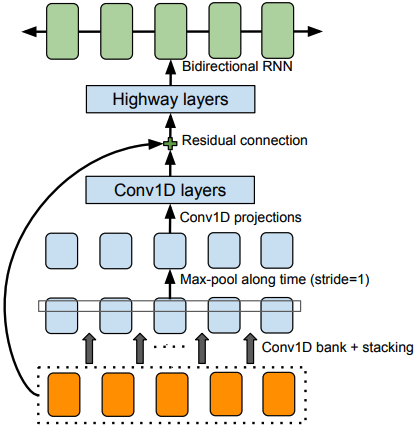
Figure 2: Lee et al. (2016)에 채택된 The CBHG (1-D convolution bank + highway network + bidirectional GRU) module
Bank of 1-D convolutional filters
- 1) 1-d conv
- 입력 시퀀스(input sequence)는 먼저 K sets의 1-D convolutional filters를 통과한다. 여기서 k번째 세트는 k너비(width)를 가지는 convolution filter
- 이러한 필터는 로컬 및 (unigrams, bigrams, up to K-grams 모델링과 유사한)contextual information(문맥정보)를 명시적으로 모델링한다.
- 2) max pooling
- convolution 출력이 함께 쌓고, local invariances를 증가시키기 위해 시간으로 max pooling한다.
- 이때 stride를 1로 사용하여 원래 time resolution을 보존한다.
- 3) fixed-width 1-D convolutions
- 4) residual connection
- 통과된 출력을 original input sequence와 더한다.
- Batch normalization은 매 convolution layer에서 사용
class BatchNormConv1d(nn.Module):
    def __init__(self, in_dim, out_dim, kernel_size, stride, padding,
                 activation=None):
        super(BatchNormConv1d, self).__init__()
        self.conv1d = nn.Conv1d(in_dim, out_dim,
                                kernel_size=kernel_size,
                                stride=stride, padding=padding, bias=False)
        self.bn = nn.BatchNorm1d(out_dim)
        self.activation = activation

    def forward(self, x):
        x = self.conv1d(x)
        if self.activation is not None:
            x = self.activation(x)
        return self.bn(x)
Highway networks
- convolution의 출력은 high level 특성을 추출하기 위해 multi-layer highway network을 통과한다.
class Highway(nn.Module):
    def __init__(self, in_size, out_size):
        super(Highway, self).__init__()
        self.H = nn.Linear(in_size, out_size)
        self.H.bias.data.zero_()
        self.T = nn.Linear(in_size, out_size)
        self.T.bias.data.fill_(-1)
        self.relu = nn.ReLU()
        self.sigmoid = nn.Sigmoid()

    def forward(self, inputs):
        H = self.relu(self.H(inputs))
        T = self.sigmoid(self.T(inputs))
        return H * T + inputs * (1.0 - T)
Bidirectional GRU RNN
- 마지막으로, forward 문맥(context)과 backward 문맥(context)에서 sequential features을 추출하기 위해서 bidirectional GRU RNN을 사용한다.
class CBHG(nn.Module):
    """CBHG module: a recurrent neural network composed of:
        - 1-d convolution banks
        - Highway networks + residual connections
        - Bidirectional gated recurrent units
    """

    def __init__(self, in_dim, K=16, projections=[128, 128]):
        super(CBHG, self).__init__()
        self.in_dim = in_dim
        self.relu = nn.ReLU()

        # A. 1-d convolution banks
        # 1)
        self.conv1d_banks = nn.ModuleList(
            [BatchNormConv1d(in_dim, in_dim, kernel_size=k, stride=1,
                             padding=k // 2, activation=self.relu)
             for k in range(1, K + 1)])
        # 2)
        self.max_pool1d = nn.MaxPool1d(kernel_size=2, stride=1, padding=1)

        in_sizes = [K * in_dim] + projections[:-1]
        activations = [self.relu] * (len(projections) - 1) + [None]

        # 3)
        self.conv1d_projections = nn.ModuleList(
            [BatchNormConv1d(in_size, out_size, kernel_size=3, stride=1,
                             padding=1, activation=ac)
             for (in_size, out_size, ac) in zip(
                 in_sizes, projections, activations)])

        # B. highway
        self.pre_highway = nn.Linear(projections[-1], in_dim, bias=False)
        self.highways = nn.ModuleList(
            [Highway(in_dim, in_dim) for _ in range(4)])

		# C. GNN
        self.gru = nn.GRU(
            in_dim, in_dim, 1, batch_first=True, bidirectional=True)

    def forward(self, inputs, input_lengths=None):
        # (B, T_in, in_dim)
        x = inputs

        # Needed to perform conv1d on time-axis # time-resolution 보존위해
        # (B, in_dim, T_in)
        if x.size(-1) == self.in_dim:
            x = x.transpose(1, 2)

        T = x.size(-1)

        # (B, in_dim*K, T_in)
        # Concat conv1d bank outputs
        x = torch.cat([conv1d(x)[:, :, :T] for conv1d in self.conv1d_banks], dim=1)
        assert x.size(1) == self.in_dim * len(self.conv1d_banks)
        x = self.max_pool1d(x)[:, :, :T]

        for conv1d in self.conv1d_projections:
            x = conv1d(x)

        # (B, T_in, in_dim)
        # Back to the original shape
        x = x.transpose(1, 2)

        if x.size(-1) != self.in_dim:
            x = self.pre_highway(x)

        # Residual connection
        x += inputs
        for highway in self.highways:
            x = highway(x)

        if input_lengths is not None:
            x = nn.utils.rnn.pack_padded_sequence(
                x, input_lengths, batch_first=True)

        # (B, T_in, in_dim*2)
        outputs, _ = self.gru(x)

        if input_lengths is not None:
            outputs, _ = nn.utils.rnn.pad_packed_sequence(
                outputs, batch_first=True)

        return outputs
- 특징
- CBHG는 machine translation에서 영감을 받았다.
- machine translation과의 차이점은 non-causal convolutions, batch normalization, residual connections, stride=1 max pooling이다.
- 이러한 modification으로 generalization 효과를 향상시켰다.
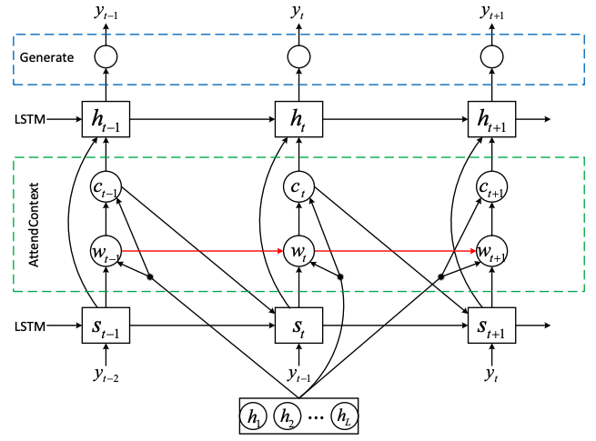
3.3 DECODER
tanh attention decoder
- 1) recurrent layer는 각 디코더 time step마다 attention query를 생성
- 2) Attention에서 나온 context vector와 RNN output concatenate해서 decoder RNN 입력
- 3) GRUs with vertical residual connections
- residual connection은 빨리 convergence될 수 있도록 도와준다.
- attention을 사용해서 Mel과 text 간의 alignment를 학습
r-frame prediction
- method
: simple fully-connected output layer 사용 - 특징
- multiple, non-overlapping output frames을 각 decoder step마다 예측.
- 장점 1) r frames을 한번에 예측하는 것은 총 decoder steps을 r로 나누고 model size, 학습 시간, 추론 시간을 단축한다.
- 장점 2) attention으로부터 학습되는 alignment가 더 빨리, 더 안정적으로 측정됨으로써 convergence speech가 증가.
- character가 보통 여러 프레임으로 구성되기 때문에 인접한 speech frames들과 correlation 높음
- 여러 프레임을 방출(Emitting)하는 것은 attention이 학습할때 더 빨리 forward로 이동하게 만든다.
- 초기값은 \ frame으로 명명하고, all-zero frame 임
- multiple, non-overlapping output frames을 각 decoder step마다 예측.
예측 Target: 80-band mel-scale spectrogram
(더 적은 bands나 cepstrum과 같은 더 간결한(concise) target을 사용할 수 있다)
-
speech signal과 text 사이에 alignment를 학습 잘 하는게 중요함.
-
raw spectrogram은 불필요한 representation이 많음. (길이 너무 길고, 용량도 너무 큼)
-
압축을 효율적으로 하기 위해서는 seq2seq output이 inversion process에 대한 prosody(운율) 정보와 sufficient intelligibility를 제공해야함.
>- 비교:
>  - Raw 스펙트로그램: 모든 주파수를 동일하게 다루기 때문에 높은 주파수에서 불필요한 정보를 많이 포함할 수 있습니다. 이는 데이터의 크기와 처리 시간을 증가시킬 수 있습니다.
>  - 80 밴드 mel-scale 스펙트로그램: 주파수 정보를 압축하여 중요한 음성 정보를 강조하는 반면, 높은 주파수에서의 세부 정보는 상대적으로 덜 표현합니다. 이로 인해 데이터는 더 작고, 처리는 더 빠르며, 효율성이 높아집니다.
class Decoder(nn.Module):
    def __init__(self, in_dim, r):
        super(Decoder, self).__init__()
        self.in_dim = in_dim
        self.r = r
        self.prenet = Prenet(in_dim * r, sizes=[256, 128])
        # (prenet_out + attention context) -> output

        # Attention RNN
        self.attention_rnn = AttentionWrapper(
            nn.GRUCell(256 + 128, 256),
            BahdanauAttention(256)
        )
        self.memory_layer = nn.Linear(256, 256, bias=False)
        self.project_to_decoder_in = nn.Linear(512, 256)

        self.decoder_rnns = nn.ModuleList(
            [nn.GRUCell(256, 256) for _ in range(2)])

        self.proj_to_mel = nn.Linear(256, in_dim * r)
        self.max_decoder_steps = 200

    def forward(self, encoder_outputs, inputs=None, memory_lengths=None):
        """
        Decoder forward step.

        If decoder inputs are not given (e.g., at testing time), as noted in
        Tacotron paper, greedy decoding is adapted.

        Args:
            encoder_outputs: Encoder outputs. (B, T_encoder, dim)
            inputs: Decoder inputs. i.e., mel-spectrogram. If None (at eval-time),
              decoder outputs are used as decoder inputs.
            memory_lengths: Encoder output (memory) lengths. If not None, used for
              attention masking.
        """
        B = encoder_outputs.size(0)

        processed_memory = self.memory_layer(encoder_outputs)
        if memory_lengths is not None:
            mask = get_mask_from_lengths(processed_memory, memory_lengths)
        else:
            mask = None

        # Run greedy decoding if inputs is None
        greedy = inputs is None

		# r-frame 단위로
        if inputs is not None:
            # Grouping multiple frames if necessary
            if inputs.size(-1) == self.in_dim:
                inputs = inputs.view(B, inputs.size(1) // self.r, -1)
            assert inputs.size(-1) == self.in_dim * self.r
            T_decoder = inputs.size(1)

        # go frames (초기값)
        initial_input = Variable(
            encoder_outputs.data.new(B, self.in_dim * self.r).zero_())

        # Init decoder states
        attention_rnn_hidden = Variable(
            encoder_outputs.data.new(B, 256).zero_())
        decoder_rnn_hiddens = [Variable(
            encoder_outputs.data.new(B, 256).zero_())
            for _ in range(len(self.decoder_rnns))]
        current_attention = Variable(
            encoder_outputs.data.new(B, 256).zero_())

        # Time first (T_decoder, B, in_dim)
        if inputs is not None:
            inputs = inputs.transpose(0, 1)

        outputs = []
        alignments = []

        t = 0
        current_input = initial_input
        while True:
            if t > 0:
                current_input = outputs[-1] if greedy else inputs[t - 1]
            # Prenet
            current_input = self.prenet(current_input)

            # Attention RNN
            attention_rnn_hidden, current_attention, alignment = self.attention_rnn(
                current_input, current_attention, attention_rnn_hidden,
                encoder_outputs, processed_memory=processed_memory, mask=mask)

            # Concat RNN output and attention context vector
            decoder_input = self.project_to_decoder_in(
                torch.cat((attention_rnn_hidden, current_attention), -1))

            # Pass through the decoder RNNs
            for idx in range(len(self.decoder_rnns)):
                decoder_rnn_hiddens[idx] = self.decoder_rnns[idx](
                    decoder_input, decoder_rnn_hiddens[idx])
                # Residual connectinon
                decoder_input = decoder_rnn_hiddens[idx] + decoder_input

            output = decoder_input
            # 80-band mel spectrogram
            output = self.proj_to_mel(output)

            outputs += [output]
            alignments += [alignment]

            t += 1

            if greedy:
                if t > 1 and is_end_of_frames(output):
                    break
                elif t > self.max_decoder_steps:
                    print("Warning! doesn't seems to be converged")
                    break
            else:
                if t >= T_decoder:
                    break

        assert greedy or len(outputs) == T_decoder

        # Back to batch first #output은 mel
        alignments = torch.stack(alignments).transpose(0, 1)
        outputs = torch.stack(outputs).transpose(0, 1).contiguous()

        return outputs, alignments
Attention
# 바다나우 어텐션 (self-attention이랑 같음)
class BahdanauAttention(nn.Module):
    def __init__(self, dim):
        super(BahdanauAttention, self).__init__()
        self.query_layer = nn.Linear(dim, dim, bias=False)
        self.tanh = nn.Tanh()
        self.v = nn.Linear(dim, 1, bias=False)

    def forward(self, query, processed_memory):
        """
        Args:
            query: (batch, 1, dim) or (batch, dim)
            processed_memory: (batch, max_time, dim)
        """
        if query.dim() == 2:
            # insert time-axis for broadcasting
            query = query.unsqueeze(1)
        # (batch, 1, dim)
        processed_query = self.query_layer(query)

        # (batch, max_time, 1)
        alignment = self.v(self.tanh(processed_query + processed_memory))

        # (batch, max_time)
        return alignment.squeeze(-1)


def get_mask_from_lengths(memory, memory_lengths):
    """Get mask tensor from list of length

    Args:
        memory: (batch, max_time, dim)
        memory_lengths: array like
    """
    mask = memory.data.new(memory.size(0), memory.size(1)).byte().zero_()
    for idx, l in enumerate(memory_lengths):
        mask[idx][:l] = 1
    return ~mask


class AttentionWrapper(nn.Module):
    def __init__(self, rnn_cell, attention_mechanism,
                 score_mask_value=-float("inf")):
        super(AttentionWrapper, self).__init__()
        self.rnn_cell = rnn_cell
        self.attention_mechanism = attention_mechanism
        self.score_mask_value = score_mask_value

    def forward(self, query, attention, cell_state, memory,
                processed_memory=None, mask=None, memory_lengths=None):

        # attention_rnn_hidden, current_attention, alignment = self.attention_rnn(
        #        current_input, current_attention, attention_rnn_hidden,
        #        encoder_outputs, processed_memory=processed_memory, mask=mask)

        if processed_memory is None:
            processed_memory = memory
        if memory_lengths is not None and mask is None:
            mask = get_mask_from_lengths(memory, memory_lengths)

        # Concat input query and previous attention context
        cell_input = torch.cat((query, attention), -1)

		# rnn에서 받은거랑 self-attention 값 concat해서 다음 rnn에 보내줌
        # Feed it to RNN
        cell_output = self.rnn_cell(cell_input, cell_state)

        # Alignment
        # (batch, max_time)
        alignment = self.attention_mechanism(cell_output, processed_memory)

        if mask is not None:
            mask = mask.view(query.size(0), -1)
            alignment.data.masked_fill_(mask, self.score_mask_value)

        # Normalize attention weight
        alignment = F.softmax(alignment)

        # Attention context vector
        # (batch, 1, dim)
        attention = torch.bmm(alignment.unsqueeze(1), memory)

        # (batch, dim)
        attention = attention.squeeze(1)

        return cell_output, attention, alignment
3.4 POST-PROCESSING NET AND WAVEFORM SYNTHESIS
POST-PROCESSING NET
-
목적:
- seq2seq target을 waveforms(파형)으로 합성할 수 있는 target으로 변환
- CBHG module 사용
-
Motivation
- Griffin-Lim 때문에, linear-frequency scale로 샘플링된 스펙트럼 크기(spectral magnitude)를 예측하도록 학습
- Full decoded sequence
- 항상 왼쪽에서 오른쪽으로 실행되는 seq2seq이랑은 달리, learnable 프레임만들어준다 ( forward,backward 정보 모두 가짐)
-
특징
- 이 모델은 vocoder parameters와 같은 alternative targets를 예측하거나 waveform 샘플을 직접 합성하는 WaveNet과 같은 neural vocoder로 사용할 수 있음
Griffin-Lim algorithm
- Griffin-Lim 알고리즘에 넣기 전에 magnitudes를 1.2제곱 하는 것은 artifacts를 감소시킨다.(harmonic enhancement 효과 때문일것이다.)
- Griffin-Lim 알고리즘이 50회 iteration을 한 후에 합리적으로 빠르게 수렴하는 것을 관찰했다.(실제로 약 30회 반복도 충분해 보인다.)
- Griffin-Lim은 미분 가능하지만(훈련 가능한 가중치가 없다) 이 과정에서 우리는 그것에 대해 어떠한 loss도 부과하지 않는다.
- Griffin-Limdm은 간단하고 이미 좋은 성능을 내지만 spectrogram to waveform inverter를 빠르고 고성능으로 학습할 수 있는 점에서 선택되었다.
Neural Vocoder 이전에 전통적인 방법의 Vocoder 기술로 Griffin-Lim 알고리즘이 있다.
Griffin-Lim 알고리즘은 Mel-spectrogram으로 계산된 STFT magnitude 값만 가지고 원본 음성을 예측하는 rule-based 알고리즘이다. 원본 음성 신호를 복원하기 위해서는 STFT magnitude 값과 STFT phase 값이 필요하기 때문에 이 phase(위상) 값을 임의로 두고 예측을 시작한다. 그렇게 예측된 음성의 STFT magnitude 값과 원래 Mel-spectrogram으로 계산된 STFT magnitude 값의 mean squared error(MSE)가 최소가 되도록 반복 수행하여 원본 음성을 찾아낸다.

#Synthesis
    # Greedy decoding
    # return mel_outputs, linear_outputs, alignments

    mel_outputs, linear_outputs, alignments = model(sequence)
    linear_output = linear_outputs[0].cpu().data.numpy()
    spectrogram = audio._denormalize(linear_output)
    alignment = alignments[0].cpu().data.numpy()

    # Predicted audio signal
    waveform = audio.inv_spectrogram(linear_output.T)

def inv_spectrogram(spectrogram):
  '''Converts spectrogram to waveform using librosa'''
  S = _db_to_amp(_denormalize(spectrogram) + hparams.ref_level_db)  # Convert back to linear
  return inv_preemphasis(_griffin_lim(S ** hparams.power))          # Reconstruct phase


def _griffin_lim(S):
  '''librosa implementation of Griffin-Lim
  Based on https://github.com/librosa/librosa/issues/434
  '''
  angles = np.exp(2j * np.pi * np.random.rand(*S.shape))
  S_complex = np.abs(S).astype(np.complex)
  y = _istft(S_complex * angles)
  for i in range(hparams.griffin_lim_iters):
    angles = np.exp(1j * np.angle(_stft(y)))
    y = _istft(S_complex * angles)
  return y
4 MODEL Setting
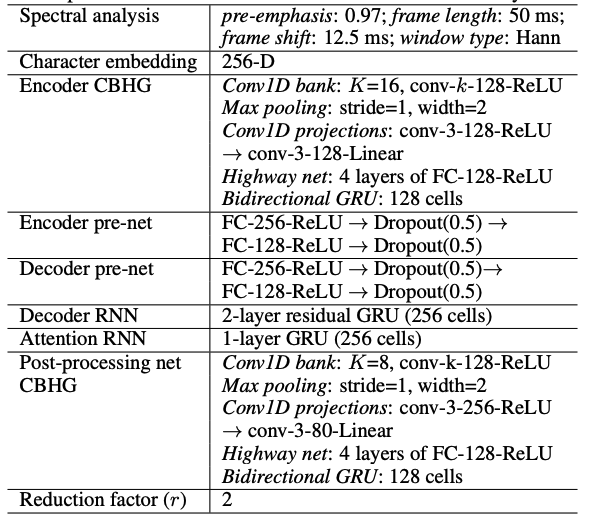
Table 1: Hyper-parameters와 network architectures. “conv-k-c-ReLU”는 ReLu activation과 함께 width와 output channels이 있는 1-D convolution을 의미한다.
- Hann windowing, 50 ms frame length, 12.5 ms frame shift, 2048-point Fourier transform(푸리에 변환)과 함께 log magnitude spectrogram을 사용한다.
- pre-emphasis (0.97)가 도움이 되는것을 발견했다.
- 모든 실험에 4 kHz sampling rate를 사용한다. 비록 더 큰 r값(e.g. r = 5)이 더 잘 작동하지만, 이 논문에서는 MOS 결과를 위해 r = 2 (output layer reduction factor)를 사용한다.
- Adam optimizer (Kingma & Ba, 2015)를 사용하고 learning rate decay는 각각 500K, 1M, 2M global steps이후, 0.001에서 시작하여 0.0005, 0.0003, 0.0001로 줄인다.
- seq2seq decoder (mel-scale spectrogram)와 post-processing net (linear-scale spectrogram) 모두에 대해 simple 1 loss을 사용한다. 두 loss는 같은 가중치를 갖는다.
- 모든 sequence는 max length에 맞춰 padding되고 32 batch size를 사용한다.
- 패딩된 부분은 zero-padded frames로 마스킹해 사용되었다.하지만 이런 방식으로 학습된 모델이 언제 emitting outputs를 멈추는지를 모르고 마지막에 반복된 소리를 만들어냈다.
- 이 문제를 해결하기 위한 한 가지 간단한 방법은 zero-padded frames을 재구성하는 것이다.
5 EXPERIMENTS
- 전문 여성 화자가 말하는 약 24.6시간의 음성 데이터를 포함하는 북미 영어 데이터 세트로 Tacotron을 학습하였다.
- 문장들은 text normalize 된다. 예를 들어 “16”은 “sixteen”으로 변환된다.
5.1 ABLATION ANALYSIS Permalink
vanilla seq2seq model 비교
-
Setting
- encoder와 decoder 모두 residual RNNs layer을 사용하며 각 layer는 256 GRU cells(LSTM을 시도했고 유사한 결과를 얻었다)을 가지고 있다.
- pre-net 또는 post-processing net를 사용하지 않았으며, decoder는 linear-scale log magnitude spectrogram를 직접 예측한다.
-
결과
-
seq2seq:
- attention이 moving forward전에 많은 프레임에 대해 고착되는 경향 (get stuck)이 있어 합성신호에서 speech intelligibility이 저하되는 원인이 된다. 그 결과 naturalness와 overall duration이 파괴된다. (뭉쳐져 있다는 건가?)
-
Tacotron은 Figure 3(c)과 같이 깨끗하고 부드러운 alignment을 학습한다.
-
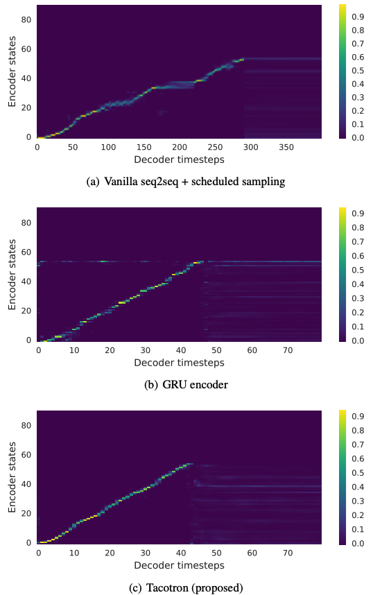
Figure 3: Attention alignments on a test phrase. Tacotron에서 decoder 길이는 output reduction factor(출력감소계수) r=5를 사용하기 때문에 더 짧다.
CBHG encoder 모델 비교
-
setting
모델의 나머지는 encoder pre-net을 포함하여 전부 같다. -
결과
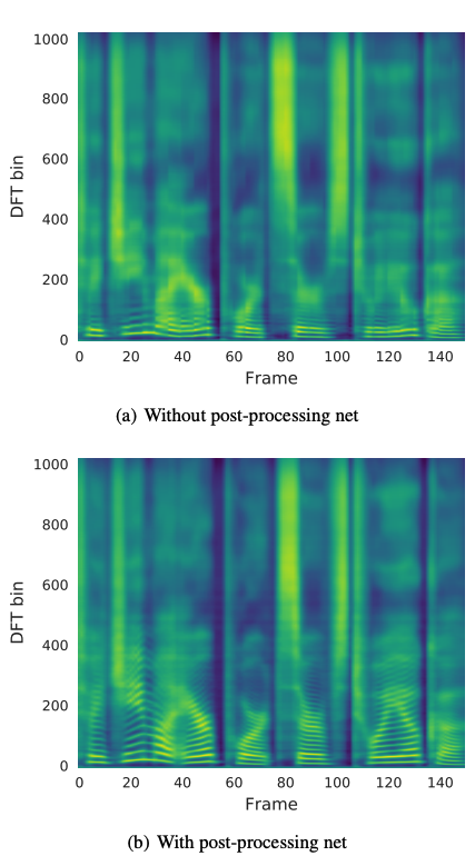
- without post-processing
- Figure 3(b)와 3(c)를 비교하면, 우리는 GRU encoder에서의 alignment가 noisier 하다는 것을 알 수 있다.
- synthesized signals(합성신호)를 들어보면, noisy alignment이 종종 잘못된 발음으로 이어진다.
- with post-processing
- CBHG encoder는 overfitting을 줄이고 길고 complex phrases(복잡한 구문)을 generalize한다.
- 더 많은 contextual information(상황별 정보)를 통해, post-processing net로부터 만들어진 prediction은 harmonics와 synthesis artifacts를 감소기키는 high frequency formant structure를 더 잘 생성한다.
- without post-processing
5.2 MEAN OPINION SCORE TESTS

- Setting
- mean opinion score test: 5 point의 리커트 척도를 사용해 자연스러움에 대해 물어봤다.
- 원어민으로부터 크라우드소싱 방식으로 모아 평가했다.
- 100개의 학습되지 않은 문장들은 테스트를 위해 사용되었고 각 문장은 총 8번의 점수를 받았다.
- MOS를 계산할 때 오직 헤드폰을 사용해서 평가한 결과만 사용하였다.
- 비교 모델
- 실제 사용되는 parametric 모델
- concatenative 모델: Google's hidden Markov model (HMM)-driven unit selection speech synthesis system (pharased base)
- 결과
- Tacotron의 MOS는 3.82로 parametric 모델 이상의 성능을 가진다.
- 강력한 baseline과 Griffin-Lim 합성에 의해 발생한 artifacts를 고려한다면, 이 결과는 매우 괜찮은 결과다.
(비교 결과 음성이 없음..) - (pharased base)랑 비교해도 나쁘지 않다 아닐까?
6 DISCUSSIONS
- Tacotron: character 시퀀스를 입력으로 받아 spectrogram을 출력하는 end-to-end TTS 모델
- 간단한 waveform 합성기 모듈과 함께 3.82의 MOS에 도달하였고, 실제 자연스러움의 부분에 있어 parametric system의 성능 능가
- Tacotron은 frame-based라서 inference가 sample-level의 autoregressive 모델에 비해 빠르다.
- 이전 연구와 달리, Tacotron은 손이 많이 가는 언어학적 특성 추출 또는 HMM aligner와 같은 복잡한 컴포넌트들이 필요하지 않다.
- 이 모델은 단순히 랜덤초기화와 함께 처음부터 학습될 수 있다.
- 학습된 text normalization에서의 최근 발전이 미래에는 text normalization을 불필요하게 할수 있겠지만, 이 모델에서는 simple text normalization을 사용하였다.
- Output layer, attention module, loss function, Griffin-Lim-based waveform synthesizer는 모두 개선 가능성이 있다.
한계
audio-text pair만 있으면 학습이 가능한 end-to-end 모델이다. 이것이 왜 가능하냐면 alignment를 attention을 통해서 학습하기 때문이다. 처음 제시한 Tacotron에서는 Bahdanau attention을 사용하였다. Alignment를 직접 학습하는 모델의 특성상 훈련 시의 alignment가 잘되면 generalization의 성능이 좋다고 한다. 그래서 학습이 잘 안될떈 local sensitve attention과 같이 다양한 시도를 해보는게 좋다고 한다.
이 계열 모델의 단점은 auto-regressive한 방식으로 frame별로 생성하기 때문에 느리다. 그리고 alignment가 잘 안되면 아무 소용이 없다. alignment를 시각화 했을 때 중간이 끊어진다던가 반복하기 쉽다고 한다.
소리비교
audio sample: https://google.github.io/tacotron/publications/tacotron/index.html
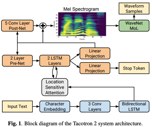
Tacotron 2: Natural TTS Synthesis by Conditioning WaveNet on Mel Spectrogram Predictions
paper: https://arxiv.org/pdf/1712.05884
audio sample: https://google.github.io/tacotron/publications/tacotron2/
code:

음절 또는 음소마다의 음성파일을 이어붙이는 방법인 Concatenative Approach

Sample code
https://pytorch.org/hub/nvidia_deeplearningexamples_tacotron2/

skip connection
수렴 속도 향상: 위의 모든 이유들로 인해, skip connection은 전반적으로 수렴 속도를 향상시키는 효과가 있습니다. 그래디언트의 효과적인 전달과 피쳐의 재사용은 모델이 더 빠르게 안정적인 성능에 도달하도록 돕습니다.